Back in episode 5 I promised to explain how to multiply matrices in a way that you probably have not seen before. I also said that I would do that within 5 episodes, and since this is now episode 10, my hands are tied.

By the way, if you are enjoying this blog, I think that you will also enjoy Dan Ghica’s wonderful series on inventing an algebraic knot theory for kids: Dan uses a similar diagrammatic language to talk about knots, but there’s one major difference between his diagrams and ours: his wires tangle! No wonder, since wires that do not tangle are not particularly useful if you want to construct knots. If you want the “real” reason, it is that his underlying mathematical structure is a braided monoidal category, whereas ours is symmetric monoidal category.

There is one more blog to mention: John Baez has recently been writing about PROPs and linear systems; check it out if you want a sneak preview of one of the star applications of graphical linear algebra! John and his student Jason Erbele developed the theory independently and more or less at the same time as Filippo, Fabio and I. But, apart from the fact that they have different conventions for drawing diagrams, the equational theory that they have developed can be shown to be equivalent to the one we will develop here. It’s super interesting that science is full of temporal coincidences like this; it’s not even the first time that this kind of thing happens to me!

---

 

 

We start by quashing the fear that the sky may fall on our heads: that is, that somehow graphical reasoning could let us do unreasonable things, like proving that 2 = 3.

Let’s convince ourselves by doing some counting, armed with a hypothetical example. Suppose we have a diagram A, say with two dangling wires on the left and one on the right. Let’s give the first left wire a name, say p and let’s call the right wire q. Suppose also that we’ve cut up the diagram into chunks, like we did with Crema di Mascarpone, and we’ve identified one particular diagram component, called B, with one dangling wire on the left, called r, and one on the right, called s. In the diagram r and s are drawn as dangling from B, but inside of A they may connect to other components.

Now how do we count the number of paths from p to q? We could write down a formula as follows.

This idea generalises easily enough; think about what happens if B has multiple dangling wires on the left and on the right. But what does all this counting tell us?

Well, for one, to count the number of paths from p to q we do not really need to look inside B, we only need to know about the number of paths from each of its dangling points on the left to each of its points on the right. In particular, if I swap B for another diagram, say C, with the same numbers of paths, then the overall number of paths from p to q will not change. The idea of counting paths is compositional.

So let’s now think about diagrammatic reasoning. Clearly stretching or tightening wires doesn’t change the number of paths. Neither does sliding generators along wires. So the only point where things could go wrong is when we use one of our equations. And what happens when we use an equation? We identify a part of the diagram, a component, that corresponds to one side of the equation, and replace it with the other. Here’s our cheat sheet again, for reference:

The thing to notice is that, in every equation, the path numbers are the same in both left and right hand side. For example, in both sides of (B1) there is one path from every dangling point on the left to every dangling point on the right. In (B2) there are no dangling points on the right, so there are no paths to speak of. In (Unit) and (Counit) there is exactly one path… and so on.

What all of this tells us is that the number of paths from any dangling point on the left to any dangling point on the right is an invariant in diagrammatic reasoning for the theory of adding and copying that we have painstakingly identified so far. So, for instance, starting with the diagram for 3 from the last episode, every diagram equal to it according to diagrammatic reasoning will have precisely three paths from the left dangling wire to the right one. In particular, this excludes the possibility of 2 being equal to 3. Phew!

---

 

In the last episode we concentrated on diagrams with precisely one dangling wire on the left and right. Let’s now broaden our horizons and draw some more complicated diagrams.

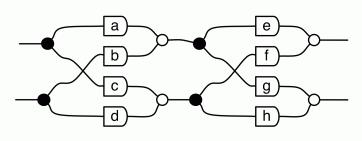
Last time I claimed that every diagram with one dangling wire at each end is equal to one that comes from the natural number syntactic sugar. We will convince ourselves of this fact soon, but for now let’s just believe that this is indeed the case. I want to compound that claim with another: there is also a general shape that describes every diagram with two dangling wires at each end. It is the following, where a, b, c and d are arbitrary natural numbers.

So, in the diagram above, there are a paths from the first dangling point on the left to the first dangling point on the right, b paths from the second on the left to the first on the right, and so on. All these fun facts almost make you want to write down a nice 2×2 square of natural numbers.

Let’s figure out what happens when we compose two such beasts; it’s an instructive exercise. We will perform a calculation to get the composition to fit into the general pattern described by the diagram above. A word of warning: the diagrams below get a bit complicated, but don’t worry, our calculations will hardly ever be this messy!

So the first thing that we do is use (B1) twice. Next we apply the (copying) lemma from the last episode four times, to bring a,b,c and d over the copying generators to their right.

Next, we use the (adding) lemma to bring e, f, g and h over the adding generators to their left, and use the (multiplying) lemma to multiply each pair.

The next thing to notice is that there are two ways of getting from the first dangling wire on the left to the first dangling wire on the right; one that goes through ea and a second that goes through fc, as indicated by the red wires in the diagram below.

The key to simplifying the diagram further is to collect all such compatible paths and add them up. At this point though, it is useful to introduce some additional syntactic sugar that will help us to reduce the complexity of our diagrams.

---

 

 

The first of our new syntactic sugars looks like the copy generator, but with three dangling wires on the right.

The reason why it’s a nice syntax is that (CoAssoc) tells us that it does not actually matter in which order we perform the copy operation, we simply end up with three equal copies.

We also introduce a sugar that looks like copy, but has four outgoing wires, as follows:

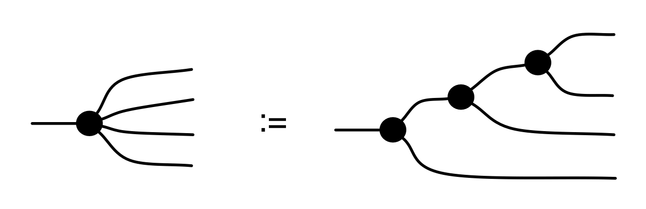
Again, the syntax is evocative, because (CoAssoc) implies that it doesn’t matter in which order we perform the copying. In particular, all of the following are equal.

We can continue this procedure recursively, obtaining a family of sugars indexed by the number of outgoing wires. The recursive case is the following:

The base case, for one outgoing wire, is simply the identity. By the way, it is also useful to consider a “copy with zero outgoing wires”, and let this be equal to the discard generator.

Next we can derive two useful laws for dealing with this family of sugars. The first one generalises (CoComm) and says that if I permute two adjacent wires then the sugar can swallow up the twist.

The equation follows from the fact that I can use (CoAssoc) to transform the diagram in such a way so that the twist connects directly to a copy generator, and then use (CoComm). Now, since any permutation whatsoever can be constructed from twist and identity using the two operations of diagrams, it follows that a copy sugar with k outputs followed by any permutation on the k wires is equal to the copy sugar: the sugar can eat up any permutation thrown at it. Simple, right? There is also a rule that generalises (CoUnit): if I cap any of the k outputs with the discard generator then the resulting diagram is the sugar with k-1 outputs. We will not use this second law for now, but it’s useful to keep in mind.

Now, since addition is bizarro copy, we can introduce a similar family of sugars for addition, which satisfy the corresponding bizarro properties that generalise (Comm) and (Unit). To get the idea, just reflect the diagrams in the explanation above and colour the circles white!

Remember the long proof of the inductive step of (copying) from last time? Using this syntactic sugar makes it much simpler. Try it! For now, we will use our sugar to simplify the rest of our current computation.

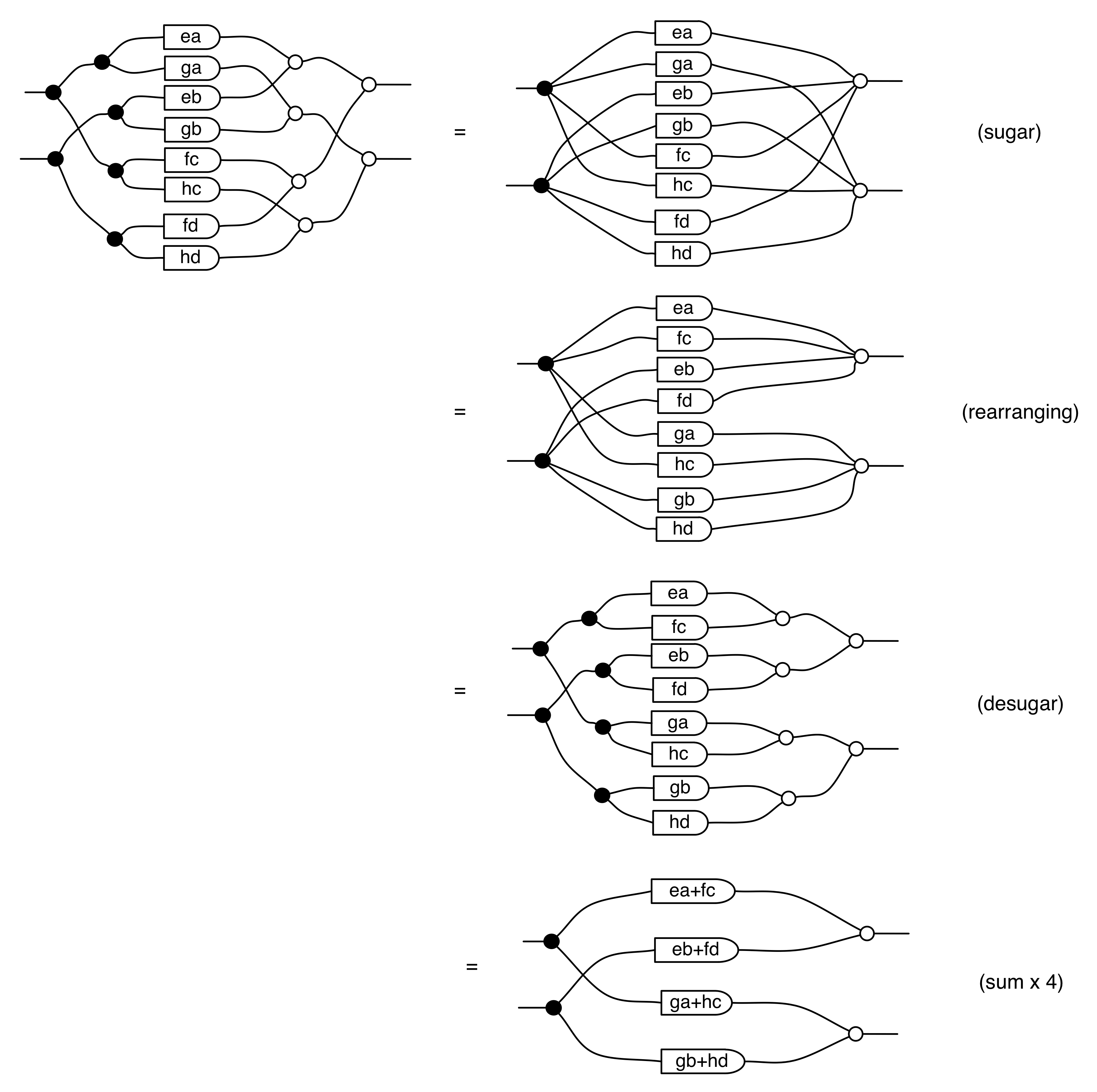
After the sugaring step, we can easily rearrange the paths by sliding numbers along wires and getting the sugars to eat up any of the resulting twists. We can then desugar into the form that allows us to apply the (sum) lemma from the last episode.

Now, if you took undergraduate linear algebra then you probably memorised the technique for multiplying 2×2 matrices. Here’s a quick reminder:

          ①

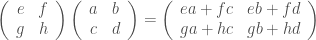
These numbers look familiar, don’t they?

In fact, the diagrams that we have been drawing all along are actually in 1-1 correspondence with matrices that have natural number entries. Moreover, just as composition of diagrams with one dangling wire at each end corresponds to multiplication of natural numbers, composing diagrams of arbitrary shape can be understood as matrix multiplication. We will go through this in more detail next time.

For now, a quick summary: the diagram

corresponds to the matrix . In general, the number of columns of the corresponding matrix is the number of dangling wires on the left, and the number of rows is the number of dangling wires on the right. Moreover, the entry at row i and column j is the number of paths from the jth wire on the left to the ith wire on the right.

Finally, the composition

corresponds to the matrix obtained by performing the matrix multiplication ①.

And, as you’ve seen, it all follows from how adding and copying interact!

Continue reading with Episode 11 – From Diagrams to Matrices