Solomon is currently a student at the University of Pennsylvania where he is pursuing a Ph.D in Computer Science. He has a keen interest in all things Computer Science and Maths, so he decided to specialize in Programming Languages, an area which applies ideas from diverse areas of Computer Science, Mathematics and Philosophy. One of his favourite things is when connections are made between seemingly disparate areas of inquiry, so he has enjoyed reading the Graphical Linear Algebra blog for the connections between string diagrams and linear algebra. As the Lindström-Gessel-Vienot Lemma shows us, there is also a surprising combinatorial connection. Such occurrences make Solomon very happy!
Consider the familiar diagram for the  matrix
  :
:

Suppose that we wanted to push some flow from the input nodes  and
and  to the output nodes
  and
and  . Moreover, we want to do this in such a way that every output node receives some flow without any congestion in the network. More specifically, want to push flow from the input nodes to the output nodes in such a way that:
- no two different paths that are part of the flow intersect at
a vertex (not even endpoints), and
- for each output node
 , there is a path from some input
node  to .
to .
For example, in the diagram above, we can push  units of flow from to and
  units of flow from to .

We can also push  units of flow from to and
  units of flow from to .
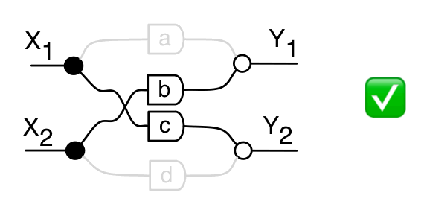
We are not allowed to push units of flow from to and units of flow from to , since then we would have two different paths intersecting at .

Also, we are not allowed to push only units of flow from to , since then there is no path from some to .

We call a flow that satisfies conditions (1) and (2) a viable flow. Now we will measure the signed weight a viable flow. The weight of a viable flow is simply the product of all weights on the edges that are part of the flow. To get the signed weight, we multiply the result by -1 if the flow links to . Otherwise, we multiply the result by +1.
For example, in our matrix example, the first viable flow has weight  . The unsigned weight of this flow is
  since we push units of flow from to and units of flow from to . To get the signed weight of this flow, we multiply the unsigned weight by +1 since is linked to . A similar computation shows that the signed weight of the second viable flow is
  .
.
Interestingly, when we add signed weights of all the viable flows in the diagram, we get the determinant of the matrix associated with the diagram i.e.  . Coincidence?
The Lindström-Gessel-Vienot Lemma (LGVL) tells us that this in fact is not a
coincidence. Specifically, LGVL associates to each finite directed acyclic
graph (dag)  a matrix whose determinant is exactly equal to the
sum of the signed weights of the viable flows in . To make this relationship precise we shall give the statement of LGVL, but first we need to introduce some definitions and notation that we will need in order to give the statement of the theorem.
First, we introduce permutations. For any sets  and
and  we call any bijection
  a permutation from
  to
to  . Now assume that
  sends
sends  to
to 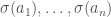 respectively. For example, let
 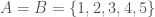 , and let send
  to
to  respectively. Write in a row in that order, skip a line, then write
  below
below  for each . Draw a line from to
  , and count the number
  of crossings in between the
  s and the
  s. Define the sign of be
  . For the permutation we have just described, there are six crossings, so the sign of the permutation is
  .
.

The sign of a permutation can also be computed by raising -1 to the
number  of inversions of , where is the number of ordered pairs
  such that
  but
but  . In the example above, the number of inversions of is 6 =
  , which gives the same result as before.
For the next few pieces of notation as well as the statement of LGVL, assume that is a finite directed acyclic graph. Assume further that has input nodes  and output nodes
  .
.
As before, we are interested in viable flows, i.e. flows that have the property that:
- no two different paths that are part of the flow intersect at
a vertex (not even endpoints), and
- for each output node
 , there is a path from some input
node to .
Each viable flow can described by an  -tuple
  of paths , where
  is a path from the input node to the output node
  for some permutation . Let
  be this permutation.
For each directed path  between any two vertices in , let
  be the product of the weights of the edges of the path. For any two vertices and , write
  for the sum

where ranges over all paths from to .
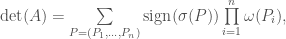
We are finally in a position to give the statement of LGVL, which is that

where ranges over all viable flows in !
LGVL holds for any finite directed acyclic graph, not just graphs that look like the example. For example consider the following graph:

or equivalently, the following string diagram:
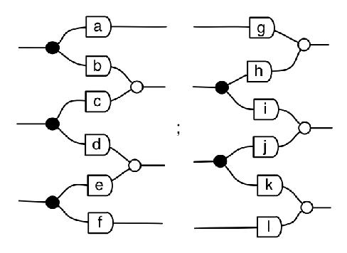
The matrix for this is

.
It has determinant  , and it is easy to check that each of these terms indeed gives a viable flow from the
  s to the
  s. Note also that the sign of each term is +1 since
  is sent to
  in each of the viable flows.
Now on the one hand, LGVL gives us a way of computing the sum of the signed weights of viable flows in a dag as the determinant of a certain matrix. On the other hand, given a matrix  , we may compute the determinant of by doing the following. First, we find a special dag . Next, we find a set of input vertices
  and output vertices
  in . We check to see that
  . Then, we (easily!) compute the sum of the signed weights of viable flows in from to . Finally we conclude that the result is equal to the determinant of by LGVL. This compositional approach to computing the determinant often leads to useful and surprising results, as we shall see below.
Consider the determinant of the following matrix:
where  denotes the greatest common divisor of
  and
and  .
.
It is difficult to come up with a closed formula for this determinant by using say row-reductions or the co-factor expansion. However, using the strategy involving LGVL gives a simple and surprising result.
But first, a few more definitions! Given any positive integer , let  denote the number of positive integers less than or equal to which are relatively prime to . For example,
  since the only numbers less than 6 that are relatively prime to 6 are 1 and 5. On the other hand
  since all the positive integers less than 7 are relatively prime to 1. In fact, it is easy to see that
  for any prime
  .
.
Also, for the purposes of the proof, we shall need to use the fact that
which is a property first established by Gauss. For example

.
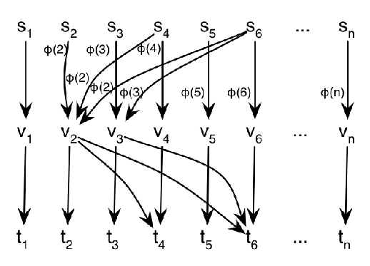
Now we proceed to the actual computation. Consider the graph which has  vertices:
  are the input vertices,
  are the output vertices and
  are intermediate vertices. If divides , put the edge
  with weight
  and the edge
  with weight 1.
What is the weight  of all the paths from
  to
to  ? Well each path from to can have only two edges: an edge
  of weight and an edge
  of weight 1, for some
  , where divides and divides . Of course the weight of this path is multiplied by 1, which is just . Therefore,
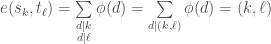
The last equality is justified by Gauss’ result.
By the LGVL, it follows that
where 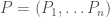 ranges over all viable flows from the input vertices
  to the output vertices
  .
.
Now the only path from  to
to  is
is  since 1 has only one divisor, namely 1. As a result, for each prime
  , any path from
  to in a viable flow must pass through
  . This is because has only two divisors, namely 1 and , but the path through 1 has already been blocked by 1.
Consequently, for any product  of two primes, any path from
  to must pass through
  . Repeating this argument for all the other numbers less than or equal to , we conclude that all the viable flows from
  to link to
  .
.
Now if there is a viable flow which links to for some  , then there must be some
  such that
  is linked to
  with
with  (why?). But this means that
  divides
  , a contradiction since
  ! So we must have
  , for all .
Thus, there is a unique viable flow from to i.e. the flow for which is sent to  via . Thus, we conclude that the determinant of is
  , since the weight of each path
  in this flow is as we showed earlier:


Cute!
LikeLike
Sweet. Thank you for sharing this!
I noticed two minor typos (omitted words) and had a few questions.
“signed weight a viable flow” –> “signed weight of a viable flow”
“Each viable flow can described by” –> “Each viable flow be can described by”
I think the variable P is overloaded between this and the following paragraphs (as both an arbitrary viable flow and an arbitrary path between two given endpoints). Am I missing something, or are these actually distinct objects?
You pass lightly over a potentially interesting point: “…given a matrix M, we may compute the determinant of M by doing the following. First, we find a special dag G…” Is this inverse operation always possible?
LikeLike
Oops. I messed up. “be can” –> “can be”. 🙂
LikeLike
”It has determinant agciek + agcifl + agdjfe + bhdjfe, and it is easy to check that each of these terms indeed gives a viable flow from the {s_i}’s to the {t_i}’s.“
should be
”It has determinant agciek + agcifl + agdjfl + bhdjfl, and it is easy to check that each of these terms indeed gives a viable flow from the {s_i}’s to the {t_i}’s.“
LikeLike
Hi Pawel. Thanks for this beautiful blog!! I have learned and enjoyed a lot.
I am a newbie on this matter. I hope someday you can explain us, in your diagrammatic picture, the characteristic polynomial and trace invariants for the Hermitian case. Are your diagrams connected with the so-called trace diagrams?: https://mathoverflow.net/questions/6139/how-can-i-learn-about-doing-linear-algebra-with-trace-diagrams
Thank you in advance !!
LikeLike