• John Baez – Semantics for open Petri nets and reaction networks
• Aleks Kissinger – Unification of the logic of causality
• Martha Lewis – Compositional approaches to linguistics and cognition
• Pawel Sobocinski – Modelling of open and interconnected systems

The data revolution of recent years means that scientific models (in physics, biology, medicine, chemistry, climate science, computer science, systems theory, …) are getting larger, more fine-grained and detailed and ever more complex. Algorithms that answer questions about model behaviour are often exponentional in the size of the model, meaning that–even with advances in hardware and software parallelisation–studying monolithic models usually does not scale. Moreover, monolithic models are poor engineering practice; for example, they are not portable in the sense that standard components cannot be reused from one application to another. These are just some of the reasons why a comprehensive mathematical theory of open and interconnected systems is urgently needed.

 

As Willems argued in The behavioral approach to open and interconnected systems, models for such systems must be fundamentally relational in order to be useful – the underlying physical equations that govern behaviour (e.g. Ohm’s law, the gas laws, …) are seldom causal: they merely govern the relationship between various system variables. This contrasts with the human custom of thinking causally about system behaviour. Willems argued that causality–while useful for human intuition–is physically dubious, not compositional and often complicates the mathematics.

 

To arrive at a comprehensive relational theory of open systems, category theory is unavoidable: one needs the generality to cover the wide variety of mathematical universes relevant in the various application areas, while identifying common structure. Carboni and Walters’ Cartesian Bicategories of relations offers a general and elegant framework for relational theories and has the potential to be relevant across multiple application areas.

1. Assemble a menagerie of relational theories from a variety of disciplines
2. Evaluate cartesian bicategories of relations as a mathematical foundation of open and interconnected systems
3. Study extensions (abelian bicategories, nonlinear variants)

 We’re delighted to announce the Applied Category Theory 2018 Adjoint School, an initiative to bring early career researchers into the applied category theory community.

 

The Adjoint School comprises two phases: (1) an online reading seminar based on the recent Kan Extension Seminars, and (2) a four day research week at the Lorentz Center, Leiden, The Netherlands. Participants will also be invited to attend Applied Category Theory 2018, which will be held immediately following the research week, also at the Lorentz Center.

During the school, participants will work under the mentorship of four mentors, on one of the following research projects: 

• John Baez: Semantics for open Petri nets and reaction networks
• Aleks Kissinger: Unification of the logic of causality
• Martha Lewis: Compositional approaches to linguistics and cognition
• Pawel Sobocinski: Modelling of open and interconnected systems

The online seminar begins in early January 2018, and will run until the research week begins on April 23rd, 2018. Applied Category Theory 2018 will be held April 30th to May 4th.

 

Applications to participate in the school are now open. For more details, including how to apply, please see here:

 

http://www.appliedcategorytheory.org/school or contact the organisers. Applications close November 1st.

 

On behalf of the organisers,

Brendan Fong (bfo@mit.edu)

Nina Otter (otter@maths.ox.ac.uk)

Last Tuesday, September 5 2017, I gave a tutorial on Graphical Linear Algebra at CONCUR 2017 the 28th International Conference on Concurrency Theory, which this year was held in Berlin.

I have a personal history with CONCUR. It was the first comp sci conference I attended (CONCUR 2001, Aalborg, Denmark). I gave my first comp sci talk the year after at a satellite event of CONCUR 2002 (Brno, Czech Republic).  Another year passed and I had a paper accepted at CONCUR 2003 (Marseille, France), even if it was mostly my brilliant coauthor’s Bartek Klin‘s  work. It was, and remains, a community with a particular way of looking at the world, and it has definitely shaped my own thinking.

So it was a real honour for me to be invited to give a tutorial at CONCUR 2017. I had a problem though: how to talk about the stuff on this blog to a community in which linear algebra is not, per se, a topic of interest.

One of the main research threads of CONCUR is process algebra. Process algebra is the study of idealised programming languages. Idealised here means two things: first, one strips away many features that would need to be included in a real-world programming language (I/O, fancy control flow, etc.) and leaves only a few fundamental ways of expressing some computational primitives, say synchronising communication, sequencing and recursion (CCS, the Calculus of Communicating Systems), or asynchronous communication with name passing, sequencing and recursion (Asynchronous π-calculus).

The basic idea is that stripping away irrelevant constructs makes a language more logically/mathematically tractable: a process algebra is thus the distillation of some computationally-inspired artefacts into a mathematically rigorous playground, allowing for the study of the expressivity of those primitives that remain and the interesting ways they interact, without interference from extraneous elements. An analogy can be made with chemistry: in order to study some fundamental reaction between compounds, one works with pure solutions in order to obtain meaningful results. That’s the basic, motivating idea, in any case.

The second meaning of the word idealised is that – unlike ordinary programming languages – process algebras allow you to write specifications as well as implementations. I won’t attempt to give a formal definition of what these words mean, but I’ll try to give some intuition.

An implementation has to be able to run: at some level of abstraction it must be able to compute outputs from inputs on some notion of computing machine. The mathematical analogy is with (total) functions X → Y. A function must be able to deal with every element of X and, given some x ∈ X, unambiguously evaluate to an element f(x) of Y.

On the other hand, a specification may be partial: it can be undefined on some inputs, where there isn’t any proscribed behaviour and the details are left to the programmer. Similarly, it may be the case that for some inputs we allow several possible results without giving any way of determining which one is preferable or how to arrive at any one particular output – this is known as non-determinism. The analogy here is with a relation R from X to Y. Since a relation is simply a subset of X×Y, it does not need to be total (i.e. there may be some x ∈ X for which there is no y ∈ Y such that (x,y) ∈ R) and it does not need to be single-valued (there may be some x ∈ X and two different elements of Y, say y₁ and y₂, with y₁≠y₂ such that both (x,y₁) and (x,y₂) are in R).

Graphical linear algebra feels like a specification language for linear algebra. Once you start using it, matrices feel like low-level implementations; the diagrammatic language gives you a higher-level way of expressing yourself. Of course, the equational theory means that we can “compile” down to the low-level stuff. A nice example of this idea in action is the diagrammatic way of dealing with the concepts of an eigenstuff (eigenspaces, eigenvalues, eigenvectors, eigenbasis) and spectral decomposition.

A linear transformation, defined by some n×n matrix A, has an eigenspace E with eigenvalue λ when for each vector v ∈ E, we have

Av = λv.

By isolating an eigenspace/eigenvalue pair (E, λ), we are saying that A has a particularly simple description on the sub-domain defined by E, where it is just scalar multiplication by λ. We can say this graphically as follows:

We will use the above equation as a diagrammatic definition of the concept of an eigenspace, eigenvalue pair (E, λ). It’s an important equality, so let’s go through the individual bits in detail.

E is a diagram from n to 0, therefore, it defines a subspace of Qⁿ. The diagram on the left is the linear relation that results from restricting the domain of A to E. Using traditional notation, the left-hand side is the linear relation

{ (e, Ae) | e ∈ E }

and the right-hand side is the linear relation

{ (e, λe) | e ∈ E }. 

The above diagrammatic equation thus says precisely that A, when restricted to E, is the same as simply multiplying by λ.

Suppose that we can find a decomposition of the entire domain (Qⁿ) of A into eigenspaces. That is, suppose we have E₁, …, E_k such that

and for each E_i, we have an eigenvalue λ_i, that is

Such a collection (E_i, λ_i) is called the spectral decomposition of A. Given a spectral decomposition, we can write A as a sum of the constituent behaviours, in the following sense:

It is useful to think of the right hand side of the equation above as a specification. Indeed, we are defining a linear transformation by declaring what it should do on each of its eigenspaces. Continuing this analogy, the left hand side is a matrix, an implementation of the specification.

Here’s a proof of the above equality, using diagrammatic reasoning. In the second step we use the third-to-last diagram above, which says that the entire domain of A can be decomposed as a sum of eigenspaces. The third step is a simple exercise in graphical linear algebra, to which we will return below. In the fourth step we pull A across the addition, and then rearrange the diagram. In the last step, we simply use the diagrammatic defining equation of eigenspaces/eigenvalues.

To dot all the i’s and cross all the t’s, let’s come back to the third equation in the above derivation. It relies on the following lemma

which can be proved by induction, starting with the following equality as the base case.

I’ll leave this last bit as a fun exercise.

Let’s go through a concrete computation that demonstrates how to turn a linear algebra specification into a matrix implementation.

So suppose we want to construct a function that acts on the following two subspaces

by multiplying by 5 and -1, respectively. In more traditional set-theory language, these subspaces are { (x,y) | x,y ∈ Q, x+2y = 0 } and { (a, 2a) | a ∈ Q }. You can read off the set theoretical descriptions directly from the diagrams by reading the first from left to right, and the second from right to left, using our standard intuitions for the meaning of the white and black dots.

Notice that the two diagrams are the colour-inverse of one another, and therefore they are orthogonal as subspaces. In general, for an implementation to result in a matrix specification, we don’t necessarily need to start with mutually orthogonal subspaces: it suffices that they add up to give the whole domain and, pairwise, have a trivial intersection, i.e.

whenever i≠j.

Since our chosen eigenvalues are 5 and -1, the first eigenspace/eigenvalue combination lets us write down the first part of the specification.

The second is then

Summing up the two components gives us the entire specification:

We should now be able to compile this thing to a matrix. Let’s start by getting the middle bit to be all black.

Now we can move the numbers out of the way

We are left with two connected black networks in the middle. Here we can use the spider theorem to simplify further.

The diagram above thus consists of a “backwards” matrix

followed by the matrix

If this is unclear, take another look at the episode that describes the connection between diagrams and matrices.

Now a “backwards” matrix, going from right to left, is the same thing as its inverse going from left to right, so the entire thing can be written as:

We can calculate the inverse in any way we like, including using graphical linear algebra. The final result of inverting and multiplying is

and this is the implementation of our original spec.

Let’s use diagrammatic reasoning to work derive the standard “textbook formula” for doing this kind of thing with matrices.

Suppose that A is an n×n matrix, and that we can find an eigenbasis: a basis of its domain Qⁿ that consists of n eigenvectors e₁, e₂, …, e_n, each e_i with eigenvalue λ_i. Using the diagrammatic definition, this means simply that:

Here it’s useful to put some numbers on the wires, to make clear that each eigenvector e_i is a column vector, i.e. a diagram from 1 to n.

Now let’s add up all of the components to get the specification for A:

We can now use diagrammatic reasoning to get this thing into something more familiar:

The last diagram can be written in matrix form. Let E be the n×n matrix with e₁,e₂, …, e_n as its column vectors. Then the first part of the final diagram above is E backwards, followed by a diagonal matrix D with the λ₁, λ₂, …, λ_n on its diagonal, finally followed by E. We therefore get the standard textbook change-of-basis formula:

This is the story I used in order to explain graphical linear algebra to people from the CONCUR community: we can think of the diagrammatic language as a specification language for linear algebra. If we pursue this analogy, as I did above, it is natural to think of matrices as implementations, implementing simple linear programs (linear transformations) on the “abstract machine” where the states come from a finite-dimensional vector space.

But graphical linear algebra is more expressive than matrices: we can give partial specifications of behaviour, as demonstrated with the diagrammatic definition of the eigenspaces/eigenvalues, as well as non-deterministic specifications. Non-determinism gives rise to the idea of refinement: how to go from a non-deterministic specification to a (non-unique) implementation that  does the job. I had a paper about this at CONCUR this year, presented by my PhD student Joshua Holland (who, by the way, applied for his PhD last year using the link on this blog!) and co-authored with Filippo Bonchi and Dusko Pavlovic. I will write more about non-determinism and refinement soon.

Last week was particularly busy. After my CONCUR tutorial in Berlin, I flew back to the UK for the inaugural STRING meeting, the 1st Workshop on String Diagrams in Computation, Logic, and Physics, which was held on Friday and Saturday (8-9 September 2017), co-located with the HDRA workshop on higher-dimensional rewriting and applications. The meeting was held in the upstairs gig area of the Jericho Tavern in Oxford.

You never know how much interest you’ll get in a brand new event, but I have to say that  it exceeded my expectations: it was a full house, with more than 60 people in the audience, enjoying an exciting programme full of great talks. I loved it.

Paul-André Mèllies giving his invited talk.

The back of the room, the Jericho was totally packed!

It was also really fun to meet a few blog readers who decided to attend. Some told me to get off my ass and write more articles. It’s definitely given me some extra motivation, so watch this space!

If you enjoyed this article, please subscribe to get email updates when new articles are published. You will find a subscription link at the bottom of this page.

This blog is currently a bit of a mess. I’ve given up–for now–on trying to keep a coherent order of episodes; eventually I will collect things and put them in the right place. But, for now, I hope that the story in this article is cute enough to stand on its own two legs.

A couple of weeks ago Robin Piedeleu left a comment in Episode 28, asking about orthogonal projections in graphical linear algebra; specifically, he asked

how would I go about forming the diagram for the orthogonal projection onto the kernel of a matrix?

This is a pretty standard exam type problem in ordinary linear algebra, and requires a fair bit of matrix hackery that one needs to memorise. I used to hate these kinds of problems, especially in exams, because I’d always make routine errors in calculations. Here, I think, the graphical notation really stands out both for pedagogical purposes and for calculation: I definitely make fewer mistakes!

This post will also be a bit quicker paced than usual because I want to get to the answer and actually perform some computations. I will omit many of the proofs, but will (quickly) explain what the concepts of orthogonality, orthogonal complements and orthogonal projections mean and how one deals with them diagrammatically.

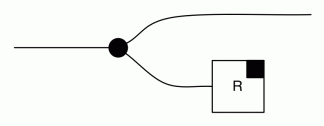
We start with a slightly different notation for arbitrary linear relations (I think due to Peter Selinger?) which is convenient for illustrating the two symmetries (colour swap and mirror image) of graphical linear algebra. Given a arbitrary diagram R: m → n, we will draw it as

The reason for this notation is that the symmetry breaking black square gives us a nice way to denote the mirror image diagram (R^†: n → m).

(Filippo, in addition, likes to mirror the letter R; I’m a bit less keen on that but it does fit the spirit.)

We can also use this notation to show the colour swap symmetry

and combine the two to get the graphical notation for bizarro (combining colour swap and mirror image) of R.

Given the quick and dirty mood of this article, I will, from now on, leave out the labels on the wires; they can be reinserted back consistently and without too much effort; leaving them out makes the diagrams cleaner and faster to draw.

The linear relations of interest for this topic will be of the form R: m → 0, which we know are just a graphical linear algebra way of saying “a subspace of Q^m“. We have a nice graphical way of denoting the sum and intersection of such subspaces. Given, R: m→0 and S: m→0, their sum R + S and intersection R ∩ S are, respectively:

The first question to tackle is what exactly does orthogonality mean, diagrammatically speaking?

Let’s start with the usual explanations. In the geometric interpretation of linear algebra, two vectors v, w are said to be orthogonal exactly when they are at right angles to each other. Algebraically, one defines the dot product of vectors:

v ⋅ w = v₁⋅w₁ + v₂⋅w₂ + … + v_m⋅w_m.

Then v and w are orthogonal exactly when v ⋅ w = 0. For example (1, 1) and (1, -1) are at right angles when we draw them in Q² and indeed, 1⋅1 + 1⋅(-1) = 0.

Given a linear subspace R, one can define the orthogonal complement of R,

R^⊥ = { v | ∀ w ∈ R. v⋅w = 0 },

which contains precisely those vectors that are orthogonal to everything in R.

The two standard facts to mention here are that R ∩ R^⊥ = {0} (the only vector that is both in R and R^⊥ is the zero vector) and R + R^⊥ = V, where V is the entire vector space. It is for this reason that R^⊥ is called a complement.

So how does this all work in graphical linear algebra?

It turns out that the answer is very easy. The orthogonal complement of R is simply its colour-inverted version. Indeed, one can show that (for any R: m→0)

which is the diagrammatic way of saying R ∩ R^⊥ = 0. Since equations in graphical linear algebra are invariant under swapping of colours (and copying/adding is commutative), we get for free that

which is the diagrammatic way of saying R + R^⊥ is everything.

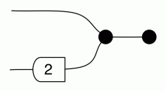
We might as well consider an example at this point. Consider the linear subspace of Q² containing pairs (x,y) such that x + 2y = 0. The diagram for this is

The orthogonal complement is the colour swapped diagram, which is the following:

Note that the scalar has changed direction – this is of course a consequence of how the sugar for natural numbers is defined, since, recall:

Colour swapping the above makes the 2 gate point the other way.

Let’s just do a quick sanity check. An example of a vector that satisfies x + 2y = 0 is (6,-3). The diagrammatic spec of the orthogonal can be read as the subspace that contains vectors of the form (a, 2a) for any a. So let’s take, e.g. a = -1, obtaining (-1,-2). Now (6,-3)⋅(-1,-2) = -6 + 6 = 0. This is not a proof, of course, but I did say that I’m skipping those today.

Ok, so now what does it mean to project orthogonally onto some linear subspace R?

It means finding a linear transformation (or, if you prefer, a matrix) A such that

Ax = x if x ∈ R and Ax = 0 if x ∈ R^⊥.

So, roughly speaking, we preserve everything in R and kill everything in its orthogonal complement. This is exactly how geometric projections work: for example if you want to project a 3D shape onto a plane. Much of the maths that underlies 3D graphics relies on this kind of linear algebra.

Now back to the story; let us construct the orthogonal projection diagrammatically.

First, consider the following diagram.

We can think of this as the linear relation that represents the partial function that acts like the identity, but restricts its domain to R. It is thus not total, because, for example, it is undefined on the orthogonal complement.

The true orthogonal projection, given something not in R, should send it to zero. Here’s another partial function that does exactly that.

Now it turns out that to get the entire thing–the orthogonal projection onto R–we just need to sum up the two cases:

which gives us the diagrammatic specification for the orthogonal projection. Let’s take the right hand side above and rewrite it into the following, more aesthetically more pleasing diagram. This is graphical linear algebra after all, and we care about diagram prettiness.

We will use the above as the diagrammatic master formula for calculating orthogonal projections.

Let’s do a couple of worked examples, e.g. projecting onto

{ (x,y) | x + 2y = 0 },

i.e.

which was our example from before. Recall that the orthogonal complement here is:

Substituting into the master equation gives

To get the actual matrix we can do a little diagrammatic calculation.

where we used the Spider Theorem (Episode 23) twice in the third step to simplify the diagram. We could continue with diagrammatic calculation, but at this point it’s quicker just to multiply the constituent matrices (and remember, the order of multiplication is “backwards”):

You may feel like doing a sanity check to see if this indeed does the job. That is, take a vector in { (x,y) | x + 2y = 0 }, which the matrix ought to leave untouched, and take one from the orthogonal complement, which the matrix must send to 0.

Just for fun, let’s quickly do the calculations for other projection, onto the orthogonal subspace.

Here the matrix is, therefore,

But Robin’s original question was about projecting onto the kernel of some matrix. And here graphical algebra has some additional pretty insights. I mentioned in a previous episode that the bizarro of a matrix (combining colour swap and mirror) is the transpose. Thus, we have, for an m×n matrix A

That is, the colour swap of a matrix is the same thing as its transpose, mirrored.

This can be quite useful. In particular consider the kernel of A.

We know that if we want the orthogonal complement we need to swap colours.

But, using our new insight, this is the same as

So the orthogonal complement of the kernel of A is the image of its transpose. Simple.

Dually, the orthogonal complement of the image of A

is

which is the same thing as

So the orthogonal complement of the image of A is the kernel of its transpose. These trivial consequences of graphical linear algebra notation are sometimes called the Fundamental Theorem of Linear Algebra.

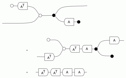
Now we can, given A, calculate a formula for the orthogonal projection onto its image. Substituting the relevant bits into the master formula gives:

From which we can read off the somewhat mysterious formula A (A^TA)^-1 A^T that appears in many linear algebra textbooks.

For the projection onto the kernel of A we get

which doesn’t obviously simplify into a “textbook formula”, but is just as easy to use in calculations.

So, since we’ve done loads of random calculations so far, let’s do one more for the road. Let’s say we want to calculate the orthogonal projection onto the kernel of

which, as a matrix is, diagrammatically

The kernel is thus

and the orthogonal complement of the kernel is

It remains to plug all the bits into the master formula for calculating projections and simplify:

which multiplies out to give

Last week I had the pleasure of visiting the Perimeter Institute for Theoretical Physics. I gave a talk about graphical linear algebra, which was recorded and available to watch online here. I emphasised the “computer science” way of looking at string diagrams as a resource sensitive syntax. That story will eventually make its way onto the blog in full, for now you can only read the beginning.

One interesting thing about the Perimeter Institute is the front entrance.

The Greek inscription translates to

Let no one uninterested in geometry enter here.

The phrase is a tribute to the phrase that was said to adorn the entrance to Plato’s Academy:

Let no one unversed in geometry enter here

I like the small change: the Perimeter Institute, in its mission statement, emphasises pedagogy as well as research.

The Perimeter Institute is the perfect research institute. It is a research factory with the best minds in theoretical physics. Crucially and refreshingly, it was built with researchers in mind. For example: there are blackboards everywhere, the open spaces encourage interactions, the architecture is inspiring and the food in the cafeteria is amazing. The contrast with 21st century British academia was… a bit depressing, and I was sad to leave.

If somebody wants to part with a few hundred million dollars, I’d love to set one up for theoretical computer science and category theory. Get in touch, philanthropic billionaires!

Aleks Kissinger and I are organising STRING 2017, a workshop for people who use, or are interested in string diagrams. The diagrams used all over this blog are an example, but string diagrams have been appearing all over the place recently: quantum computing, logic, asynchronous circuit analysis, and even linguistics. I’m trying to write a few articles about why this is happening, so if you’re interested, here’s a link to the first part.

I’m pretty excited about the workshop: first, the venue is amazing, it’s the Jericho Tavern (or more precisely, the upstairs concert venue, famous for being the place where Radiohead, while still at uni, had their (first?) gig. I’ve been to one workshop there before, in October 2014, and it was great: the atmosphere is informal, comfortable, and very conducive to discussions. At that workshop I talked about my initial ideas for graphical linear algebra, and had some really useful feedback. So I’m looking forward to going back.

Second, we have some really fantastic invited speakers: Paul-André Mèllies is coming from Paris to talk about his research on logic, which heavily features the use of string diagrams. His work on logical negation is particularly interesting. He’s the modern day Charles Sanders Peirce, who was doing logic with string diagrams (existential graphs) before Frege did it with classical syntax.

Next, Dan Ghica will give a tutorial on applications of string diagrams in circuit design and verification. His work is related but somewhat different from the graphical linear algebra kinds of diagrams, which Filippo, Fabio and I have been using for signal flow graphs. If you don’t know the details of Dan’s latest work, you might remember him from his articles about developing knot theory for eight year olds.

Finally, Bob Coecke, one of the founders of the string-diagrams-as-syntax-for-quantum-physics school of thought, will give a tutorial on the quantum applications. And possibly, perform in the evening as part of The Quantum Dagger Orchestra.

We are soliciting short abstracts, so please consider submitting something: the deadline is end of June, so there is plenty of time. Of course, you can also come along without presenting anything and simply soak up the string diagrammatic goodness. You’ll be able to register at the FSCD website when they eventually put up a registration link; I don’t remember the exact numbers but the whole thing should cost between £100 and £150, with catering included. You’ll have to pay for your own beer, of course (soft drinks are also available, I’m told). The official call for papers with all the details is below.

CALL FOR PAPERS
1st Annual Workshop on String Diagrams in
Computation, Logic, and Physics
(STRING 2017)

http://string2017.cs.ru.nl/index.html

Satellite workshop of FSCD 2017,
co-located with HDRA 2017.

Jericho Tavern, Oxford, UK
September 8-9, 2017

String diagrams are a powerful tool for reasoning about processes and composition. Originally developed as a convenient notation for the arrows of monoidal and higher categories, they are increasingly used in the formal study of digital circuits, control theory, concurrency, quantum and classical computation, natural language processes, logic and more. String diagrams combine the advantages of formal syntax with intuitive aspects: the graphical nature of terms means that they often reflect the topology of systems under consideration. Moreover, diagrammatic reasoning transforms formal arguments into dynamic, moving images, thus building domain specific intuitions, valuable both for practitioners and pedagogy.

This workshop aims to bring together researchers from diverse backgrounds and specialities to collaborate and share their insights, tools, and techniques. It will furthermore provide an informal atmosphere in a unique venue: the upstairs of the Jericho Tavern, a music venue, where famously Radiohead played their first concert. All the usual conference facilities will be provided, and the distinctive location will provide plenty of opportunities to discuss and share ideas. STRING 2017 is a satellite event of FSCD 2017 (http://www.cs.ox.ac.uk/conferences/fscd2017/) and will be co-located with the 3rd Higher-Dimensional Rewriting and Applications (http://hdra.gforge.inria.fr).

Invited Speakers

• Paul-André Mèllies (CNRS and Paris Diderot) – joint HDRA and STRING invited speaker
• Dan Ghica (Birmingham) – applications of string diagrams in circuit design and verification
• Bob Coecke (Oxford) – applications of string diagrams in quantum foundations and quantum computation

Submitting

We warmly welcome all types of contributions, ranging from work-in-progress to original work and/or overviews of mature work published elsewhere, on topics ranging from theory of string diagrams, to applications and tool demos.

Prospective speakers are invited to submit a title and 2 page abstract via the Easychair page at https://easychair.org/conferences/?conf=string2017

We will try to build a programme that is as inclusive and wide-ranging as possible within the fairly limited time available. Hence, speakers will be invited either to give a full-length talk or give a short talk in a “lightning session” style format.

The accepted abstracts will be made available electronically before the workshop.

Important Dates

Abstract deadline: 30 June 2017
Speaker notification: 14 July 2017
Workshop: 8-9 September 2017

Program Committee

• Filippo Bonchi (ENS Lyon)
• Ross Duncan (Strathclyde)
• Fabio Gadducci (Pisa)
• Aleks Kissinger (Radboud)
• Dan Marsden (Oxford)
• Mehrnoosh Sadrzadeh (Queen Mary)
• Pawel Sobocinski (Southampton)
• David Spivak (MIT)
• Noam Zeilberger (Birmingham)

Organisers

• Aleks Kissinger – Radboud Universiteit
• Pawel Sobocinski – University of Southampton

Publicity

• Joshua Holland – University of Southampton

Sometimes I put the URL of this blog into a search engine to see what people are saying. When I first started – having heard about the fabled Internet Hate Machine – I was a little worried that I’d have to deal with tons snarky remarks and negativity. The opposite has happened. I’ve received several touching personal “thank you” emails, and a large majority – maybe even 90% – of social media feedback has been positive and extremely polite.  So, unexpectedly, it’s been a bit of an Internet Love Fest. It’s all a bit disconcerting: hey, I enjoy arguments as much as the next guy!

Of the non-positive 10% of remarks, 95% have been quite useful and constructive. They allowed me to look outside my own conceptual bubble and understand the parts of blog that people have found mysterious, unclear or even annoying. In particular, there is one recurring sentiment.

The guy has some interesting insights, but what’s that weird diagrammatic notation all about?

I realised that I spent a lot of time talking about “the rules of the game” for dealing with string diagrams, using them in proofs and explaining some technical facts about what they mean mathematically, but I never really explained the fundamental questions of why people should care about them. This made me re-evaluate the way I present this material: at the recent Midlands Graduate School I spent half of my four lectures explaining the story of string diagrams and why computer scientists (and engineers, physicists, mathematicians, economists, philosophers,…) ought to care about them.

I think that this is an important missing chapter of the story so far. It’s an interesting tale in itself, involving natural language, Universal Algebra, programming languages and higher category theory. I will make the case that string diagrams are not only important, they’re inevitable. And it’s due to something called resource-sensitivity.

What is resource-sensitivity?

It’s a cliché that the digital revolution has changed the way we understand the world. One, somewhat under appreciated aspect is the way that the concept of data has changed the way human beings perceive reality.  Sequences of 0s and 1s encode all kinds of information and have spoiled us: millenia of experience of coping with finiteness (food, money, time, etc.) has been augmented with an immensely powerful resource that comes with an unprecedented ability to be copied and thrown away at will. Media companies have been struggling with this disturbing new reality since the days of Napster. Dealing with data is also a conceptual leap that programmers have to make when first learning to program; they learn to navigate this unfamiliar and exotic world, governed by a resource like few other in human experience.

Let’s start with a simple example of resource-insensitivity. The following is a very simple function, in C syntax, that takes an integer x, multiplies it by itself, and returns the result.

int square (int x) {
    return x * x;
}

The same identifier x appears twice in the body of the function (and another time, at the start, where it’s declared as the parameter). That means that the resource that the function deals with, in this case an integer, is implicitly assumed to be copyable. This is fine: an integer is represented by a sequence of 0s and 1s in memory. It’s not a problem to use it several times, copy it somewhere else or even overwrite it.

But not every resource is as permissive as data. One of the first string diagrams on this blog was the recipe for Crema di Mascarpone. The wires were typed with ingredients and there were several generators; for example a crack-egg generator that took an egg and produced a white and a yolk.

Actually, it was subsequently criticised by a colleague on my Facebook for not being truly honest, because it implicitly threw away the shell. But here’s something less controversial: I think everyone would agree that doesn’t make sense to include an egg-copy generator.

So, while copying numbers is ok, copying eggs is not. It’s an amusing idea precisely because we are intuitively aware of the concept of resource-sensitivity. Actually, once you start thinking about it, there are examples everywhere. For example consider the following, grammatically correct sentence in a natural language:

Have your cake and eat it too.

This aphorism is used in situations where you can’t have something both ways. But the literal meaning is referring to a physical object: you can’t have a physical cake, eat it and still have it, since the action of eating it destroys it. So, perhaps, a hypothetical programming lanuage for cake handling should not allow you to write the following routine:

cake handle_cake (cake c) {
    eat c;
    return c;
}

Here executing the command eat c; consumes the resource c, so there is nothing to return.  It seems that type cake is quite unlike the type int of integers.  We will call the integer kind of data classical: classical data can be copied and discarded, whereas non-classical data (like eggs and cakes) cannot.

The closest thing to classical data that we had before computers is referencing things or concepts. In other words, information, which can be copied (e.g. by monks) and discarded (e.g. in a bonfire). Natural languages like English evolved to express information, and so they have several classical features built-in. In particular, the way that sentences of natural language are constructed are an example of something called classical syntax. Classical syntax is a good fit for dealing with classical data like information, but as we will see, also has some annoying limitations.

What is classical syntax?

Trees are a popular way of organising classical data, and are closely related to the notion of classical syntax.

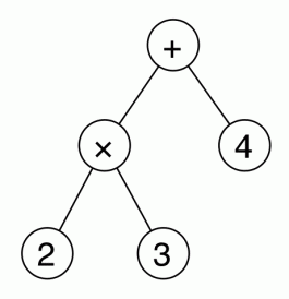
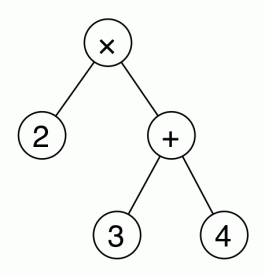
Unlike traditional trees, like the Hawaiian one in the photo above, abstract trees are usually drawn with the root at the top. For example, the following is the tree representation of the expression 2 × 3 + 4.

The usual convention that × is evaluated before + is captured by the fact that × appears deeper in the tree than +. So actually, trees are better than formulas because they eliminate the need for parentheses. For example, the tree for 2 × (3 + 4) is the following:

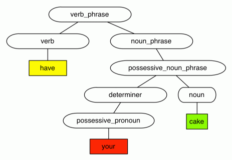
Expressions in natural language such as “you can’t have your cake and eat it too” can also be represented as trees. A lot of this is due to work by Noam Chomsky on the theory of context free grammars (CFGs), although some people date work on CFGs and their relationship with natural language back to ancient India. So “have your cake” looks something like this, as a syntax tree:

(Don’t trust me, I never actually studied English grammar. When I went to high school in Australia back in the 90s, teaching formal grammar was unfashionable and considered to “stifle creativity”. What a load of…)

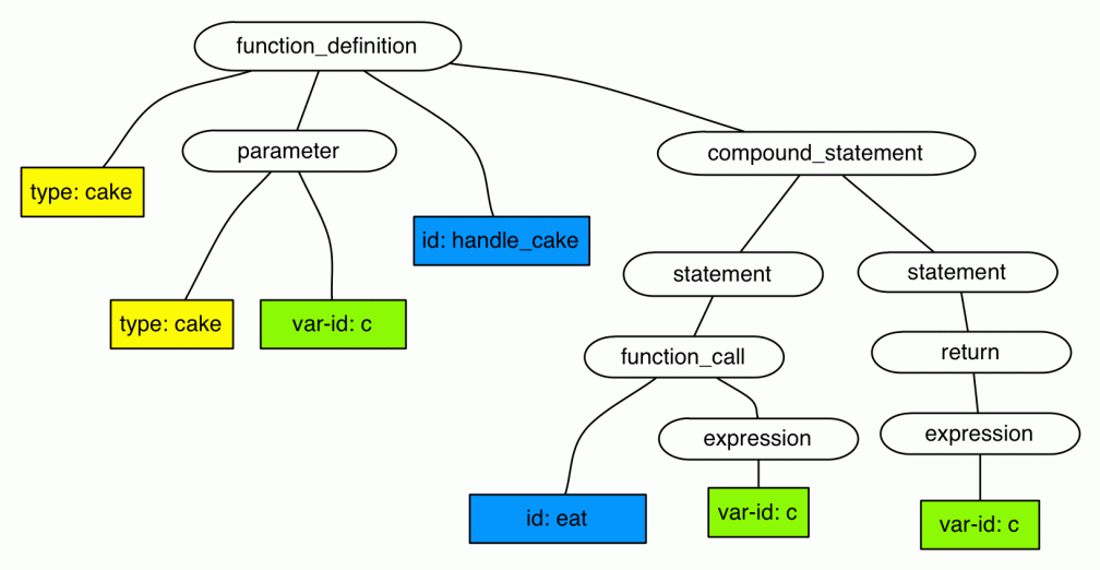
Anyway, as you can see from the tree above, natural language grammars are complicated things. CFGs are also used to define the syntax of programming languages; fortunately, these are actually much simpler to describe than natural language grammars, which are full of exceptions and special cases. So here’s how the cake handling program from before might look like as a tree:

This is roughly the kind of tree that’s constructed by the compiler, or, more precisely, by one of its components, the parser. Here I’m being somewhat reductive: in the programming language context such trees have special features to deal with variables and identifiers, and these kinds of extended trees are referred to as abstract syntax.

The cake c is referred to twice in the body of the function and once in the declaration.  But since cake is a non-classical, resource-sensitive type, then perhaps the compiler ought to ensure that the variable appears only once in the function body? So maybe our cake programming language should reject this program as a syntax error?

This doesn’t really work very well. For example, some actions might preserve the resource. For example, following ought to be ok: there’s no problem with looking at your cake and having it too.

cake handle_cake (cake c) {
    look_at c;
    return c;
}

One popular way to go about solving this problem is to build a little type theory for cakes and catch these kinds of bugs during type checking. Although this often works, is often very cute, and is quite similar to the kind of semantic analysis that goes on in our heads when trying to make sense of expressions in natural language, I think that it ignores a deeper issue:  we are cramming non-classical data into classical syntax.

Other interesting repercussions that will become clear when we think about the mathematics that governs the behaviour of classical syntax. More about this next time. For now, I’ll highlight some things that I think are symptoms of the widespread disease of classical thinking about non-classical things.

Limitations of classical thinking

Apart from cakes, here are some other examples of non-classical data, in order of decreasing coolness:  qubits, money and time. In fact, almost any finite resource you can think of is non-classical, and they all pose similar problems. All these examples are of things that, like eggs and unlike information, cannot be arbitrarily copied and discarded.

But even for ordinary, classical 0s and 1s kind of data, sometimes resource-sensitivity comes into play. A good example is concurrency: the idea that a computation can be split into a number of threads that are executed in parallel. The threads then maybe communicate and synchronise several times during processing in order to perform a task faster than would be possible when using a single thread.

Concurrent programming is the the task of writing programs that can do several things at the same time. It is more important and necessary then ever before, because hardware has been getting increasingly parallel in the last 15 years. Unfortunately, it is also widely feared and considered to be extremely hard to get right. Here, although the data is classical, the actual act of computation is resource-sensitive.  Two or more threads accessing and modyifying the same piece of data can have weird consequences, because of the non-determinism: we can’t predict before hand which thread will get to the data first, and it quickly becomes infeasible to examine all the possibilities.  Getting this wrong can sometimes have deadly consequences. I’ll return to the topic of concurrency later because it’s one of my favourite things to talk about. For now, I will tell you my own personal hypothesis: one of the main reasons why programming language technology has problems with concurrency is that ordinary, classical syntax has problems dealing with resource-sensitive applications such as concurrency. I think that string diagrams can help. (Incidentally, I recently watched Bartosz Milewski’s introduction to category theory lectures:  it was extremely cool to see someone introducing category theory and talking about programming in general, and concurrency in particular! I highly recommend the videos.)

Finally, one of the main points of this blog is that resource-sensitive thinking can actually help in areas that have traditionally been understood in a resource-insensitive way. For example, doing linear algebra with string diagrams reveals all kinds of beautiful symmetries that are hidden or only half visible when expressed in traditional, classical language. This is because the copying and discarding is explicitly a part of the graphical lexicon – it is the black structure of interacting Hopf monoids. Here, although the data is classical, it is nevertheless useful to be explicit about when the copying and discarding is done: only then the full picture becomes visible.

This episode has turned into one long piece of motivational text, with not too much technical content. This will change, because there is quite a bit of nice mathematics involved. So, my plans in the next few episodes are to answer the following questions in more detail:

• what are the mathematical properties of classical syntax?
• how can classical syntax be made (more) resource-sensitive?
• what is true resource-sensitive syntax? (spoiler: it’s string diagrams, just like the ones all over this blog!)
• how to convert classical syntax to resource-sensitive syntax?
• what are some examples of classical syntax, viewed through resource-sensitive glasses?
• what is the history of string diagrams?
• what are some future research and technological challenges to be solved?

The moral of the story will be that string diagrams are not just some weird, trendy notation. They are inevitable, once we accept that the world is full of non-classical things that need to be described properly. String diagrams are resource-sensitive syntax.

In the last few months I taught three graduate mini-courses about string diagrams and graphical linear algebra – at Phd Open in Warsaw, a winter school in Estonia, and a graduate school in Leicester. That and teaching have been keeping me busy, so I haven’t invested as much time as I would have liked on the blog. There was also the need to write down all the work done in Hawaii, and Dusko, Filippo and I just finished writing a meaty technical report, which will soon appear on the arXiv. The time that I actually did spent writing blog stuff was distributed across a number of different articles; so now I have a whole bunch of half-finished stuff. I really need to start managing this whole project a little better!

Here’s something really short and off the cuff. At MGS in Leicester, during the exercise sessions, I talked about distributive laws of props. At the same graduate school, Alexander Kurz was giving a course on category theory.  I got the inspiration for this article from one of his lectures.

As part of the distributive laws of props story, you realise that categories are a special case of the concept of monad. But monads are a special case of the concept of monoid. And monoids–of course–are a special case of the concept of category. By transitivity of the “special case of” relation, we should therefore probably just admit that they are all really the same thing: some kind of Platonic form of plugging things into each other. The story is full of pleasant categorical mental gymnastics. Think of it as the categorical equivalent of a 5km fun run.

… , a monoid is a category, …

A category is a collection of objects and arrows. Every object has an identity arrow, and any pair arrows f: A → B, g: B → C, where f‘s codomain is the same as g‘s domain, can be composed. Composition is associative, and composing with identities does nothing.

If we restrict to categories with exactly one object – let’s give it a name, say * – there is just one identity arrow  (the identity id_* on *). Every arrow has * as both domain and codomain, since there are no other objects around. So every arrow can be composed with every other arrow. Composition is associative, and composing with id_* on either side leaves any arrow unchanged. In other words, there is a set of arrows Ar with a total, associative, unital operation: i.e. a monoid. The fact that there is an object * adds no interesting information.

So every monoid is a kind of category, a category with one object. Categories, it would seem, are the more general concept. Indeed, some people say that categories are the “categorification” of the concept of monoid. Maybe categories should actually have been called monoidoids?

… , a category is a monad, …

One way to define the concept of monad is as a triple (T, μ, η), where T: C → C is an endofunctor, μ: T² → T is the multiplication natural transformation, and η: 1 → C is the unit natural transformation. Multiplication μ is associative and has η as unit, which is usually said with the aid of three commutative diagrams.

In the famous paper 1970s paper “The formal theory of monads“, Ross Street realised that this popular definition is unnecessarily specific. There’s no reason to be overly specific in mathematics: if you can easily have a more general theory/theorems, then why not? What matters is getting to the core of the issues, and not getting too hung up on extraneous details.

In this specific case, an endofunctor is a 1-cell in the 2-category Cat of categories, functors, and natural transformations. The data defining a monad is thus one 1-cell and two 2-cells, subject to some commutative diagrams of 2-cells. The fact that this data lives in Cat brings nothing important to the story: the definition clearly makes sense in any 2-category.

The 2-category Span(Set) is one of my favourites. It’s actually a bicategory–composition is not strictly associative, but we will ignore that detail for the purposes of this lightning article. It’s really just a bit of bureaucracy and adds nothing to the story. Trust me.

The objects of Span(Set) are sets. The arrows from X to Y are spans of functions

X ← Z → Y

Identities are spans formed of two identity functions. Composition of spans involves taking pullbacks. Finally, the 2-cells are span morphisms; functions Z→Z’ that make the two resulting triangles commute. I won’t bore you with the details which you can find on nlab.

The interesting question is what happens when we consider a monad in Span(Set). An endo-1-cell is span of the form

X ← Y → X                           (†).

Let’s call the left function δ₀ and the right δ₁. Now we need to give two 2-cells, that is, morphisms of spans. Let’s do the unit first: when you unpack the definitions it is a function

ι: X → Y such that δ₀ιx = δ₁ιx = x.

The multiplication μ goes from the span composed with itself back to itself. When you compute the composition, taking the pullback, the span is

X ← Y×_XY → X

where Y×_XY = { (y,y’) | δ₁(y) = δ₀(y’) }. So μ: Y×_XY → Y, satisfying δ₀μ(y, y’) = δ₀y and δ₁μ(y, y’) = δ₁y’.

So far so good. Associativity says simply that μ(μ(y, y’), y”) = μ(y, μ(y’, y”)) and the unit conditions say that μ(y, ιδ₁ y) = y = μ( ιδ₀y, y).

All this data has another name: a category. Let’s make it clearer with more familiar terminology: X is the set of objects, Y is the set of arrows. δ₀ and δ₁ give, respectively, the domain and codomain of each arrow. The function ι: X→Y picks out the identity arrows. Next, Y×_XY is the set of composable arrows, and μ: Y×_XY → Y defines the composition for any composable pair. The remaining conditions say exactly that composition is associative and identities work as they should. It’s precisely the data we need.

So, a category is just a special case of the more general concept of monad, right?

… , a monad is a monoid, …

Not so fast. We talked about monads in the generality of 2-categories. The theory of monoids can be easily generalised too: there’s no reason for the specificity of  “set” M, with unit “element” e and multiplication “function” m, satisfying associativity and the unit equations. The world would be boring if everything was just sets and functions. In fact, the concept of monoid makes sense in any monoidal category. Pick some monoidal category X; the data of a monoid consists of

an object X, and arrows m: X⊗X → X and e: I → X

where I is the monoidal unit object. Associativity and the unit laws can be expressed as three commutative diagrams. The usual monoid-as-a-set version is now a monoid, in the more general sense, instantiated in the monoidal category of sets and functions Set_×. Here the cartesian product serves as monoidal product.

So now let’s consider some 2-category C, pick an object C ∈ C and focus on the set of 1-cells from C to C. Let’s call this thing [C, C]. Actually, it’s not really a set: it’s the full sub-2-category of C on C; i.e. a 2-category with one object. We saw before that to give a category with one object is to give a monoid. In the same spirit, a 2-category with one object has the same information as a (strict) monoidal category. The objects are the 1-cells, and monoidal product (on 1-cells) is composition. I’ll leave the remaining details as a simple exercise.

So what is a monoid in [C, C], considered as a monoidal category? You guessed it – it’s a monad.

So monads are really special kinds of monoids. And monoids are really special kinds of categories. And categories are really special kinds of monads. And …

Chapter 12 of Fibonacci’s Liber Abaci is full of compelling problems. One is called “On two men with fish and the customs agent”. Another is a riddle about a man who visits a pleasure garden – accessible through seven guarded doors – where it’s possible to collect apples. You can enter freely, but on your way out you must pay each of the seven guards a tax: half of the apples you’re carrying, plus one additional apple.

Artistic impression of Fibonacci’s pleasure garden. The tax at this door is ¹⁰/₂ + 1 = 6 apples.

So, Fibonacci asks, how may apples does the man need to collect in the pleasure garden so that he gets to take one apple home? (spoiler: 382).

Given Fibonacci’s trading roots, his obsession with tax and customs duties is understandable. Without doubt, however, the most famous part of the chapter is not about taxes. It’s a very short exposition entitled “How many pairs of rabbits are created by one pair in one year”, and it starts as follows:

A certain man had one pair of rabbits together in a certain enclosed place, and one wishes to know how many are created from the pair in one year when it is the nature of them in a single month to bear another pair, and in the second month those born to bear also.

Fibonacci doesn’t tell us the name of the certain man. It will become boring to refer to him repeatedly as “the certain man”, so from now on we will change his gender to female and refer to her as Giusy (pronounced Juicy), short for Giuseppa the Rabbit Breeder.

The following helpful table is included in the margin, with the number of rabbit pairs for each month

	beginning	1
	first	2
	second	3
	third	5
	fourth	8
	fifth	13
	sixth	21
	seventh	34
	eighth	55
	ninth	89
	tenth	144
	eleventh	233
	twelfth	377

and the procedure for calculating the successive entries is explained as follows

You can indeed see in the margin how we operated, namely that we added the first number to the second, namely the 1 to the 2, and the second to the third, and the third to the fourth, and the fourth to the fifth, and thus one after another until we added the tenth to the eleventh, namely the 144 to the 233, and we had the above written sum of rabbits, namely 377, and thus you can in order find it for an unending number of months.

This sequence of numbers in the table

1, 2, 3, 5, 8, 13, 21, 34, 55, 89, …                          ①

is now known as the Fibonacci numbers. As Fibonacci explains, starting with F₀ = 1 and F₁ = 2, we obtain successive entries by recursively calculating

F_n+2 = F_n+1 + F_n.

This famous series—and the related golden ratio–are the absolute bread and butter of popular mathematics. Many facts, factoids and myths involving pineapples, pine cones, aesthetically pleasing rectangles, renaissance paintings etc. have been assigned to them.  They spice up the otherwise vapid pages of Dan Brown novels. As well as books, there are hundreds of videos on YouTube. While many are terrible, there are some gems: for example, this lecture by Keith Devlin is very good since he manages to be engaging, while at the same time challenging some of the most egregious numerological pseudo-science.

In modern presentations, Fibonacci’s famous sequence is usually given as

0, 1, 1, 2, 3, 5, 8, 13, 21, …                              ②

or

1, 1, 2, 3, 5, 8, 13, 21, 34, …                            ③

We will stick with Fibonacci’s original version ①.  There’s a good reason for this: Giusy’s first couple of rabbits start breeding already in the first month. So if the first rabbit couple was delivered one month late, Giusy would observe the following series

0, 1, 2, 3, 5, 8, 13, 21, …                               ④

Fibonacci’s ① starts with the third number of ② and the second of ③.  But it wouldn’t really work to simply shift ② or ③ to the left: differently from ④, both ② and ③ contain the sequence 1, 1, which Giusy would never observe.

We can obtain ① by adding ② and ③. Addition works pointwise, scanning vertically, 0+1=1, 1+1=2, 1+2=3 etc, as illustrated below. As we will see, this is the way of defining addition on number sequences. We will also define multiplication on sequences, but it won’t work anything like this.

The story of graphical linear algebra so far has taken us from zero to the natural numbers, to integers and then fractions. For the next few episodes we will shift our focus of from numbers to sequences. My aim for the rest of this episode is to whet your appetite by giving you a taste of the maths that we will use. For now, it will be a high-level overview, we will not go over everything in detail.

Eventually we will discuss some applications in control theory and I will do my best to explain when we come to that, although I’m not an expert. In this episode, though, I’ll talk about computer science motivations; some of the things that I found the most interesting while playing around in this particular neck of the graphical linear algebra woods.

We start by generalising Fibonacci’s rabbit problem.

Giusy originally got a pair of rabbits. No external rabbits get added, nor any taken away at any point afterwards. So we can think of this as the following rabbit input sequence

1, 0, 0, 0, 0, 0, 0, 0, 0, 0, …

with resulting rabbit output sequence

1, 2, 3, 5, 8, 13, 21, 34, 55, 89, …

Similarly, as we have already discussed, adding the first pair one month late would mean that the shifted rabbit input sequence

0, 1, 0, 0, 0, 0, 0, 0, 0, 0, …

results in the shifted output sequence

0, 1, 2, 3, 5, 8, 13, 21, 34, 55, …

But there’s no reason to add just one pair. For example, what if Giusy started with two pairs of rabbits? And, moreover, let’s suppose that she goes to the rabbit market every second month to buy another pair of rabbits. This rabbit input sequence would then be

2, 0, 1, 0, 1, 0, 1, 0, 1, 0, …                           ⑤

Following the Fibonacci principle of rabbit reproduction, we would get output sequence

2, 4, 7, 12, 20, 33, 54, 88, 143, 232, …       ⑥

The reasoning is as follows: the input sequence 2, 0, 0, 0, 0, … produces the result 2, 4, 6, 10, 16, … obtained by doubling each entry of ①. Twice the rabbits, twice the breeding. Next, 0, 0, 1, 0, 0, 0, 0, … produces 0, 0, 1, 2, 3, 5, …; that is, a shifted ①. Similarly for 0, 0, 0, 0, 1, 0, 0, 0, 0, … and so forth. Adding up all of these input sequences results in ⑤, so adding up all of the result sequences results in ⑥.

We can use the same kind of reasoning to figure out what would happen if Giusy started an ambitious commercial rabbit breeding farm. Say her business plan started with investing in three pairs, then selling one pair in the first month, two in the second, three in the third, and so forth. In this case, the rabbit input sequence would be

3, -1, -2, -3, -4, -5, -6, -7, -8, -9, …

and the result is, unfortunately

3, 5, 5, 5, 3, -1, -9, -23, -47, -87, …

so it looks like Giusy’s rabbit business would collapse sometime in the fifth month: negative rabbits doesn’t sound good. To be a successful rabbit entrepreneur, Giusy needs to understand the principles of sustainable rabbit farming, which we will discover at the end of this episode.

What’s going on here, mathematically speaking?

It looks like we are defining a function that takes number sequences to number sequences. By introducing and taking away rabbits we are causing the total numbers to change. We could try to write down a formula to calculate subsequent entries in the output sequence based on previously outputted values and the current input value. But formulas are boring.

Moreover, I hope that I’ve managed to make you at least a little bit uncomfortable about the pseudo-scientific language of causality. In graphical linear algebra, relations take centre stage. Of course, it is useful to know when a relation describes a function – as we will see below – but functions are not part of our basic setup. Instead, we think of the Fibonacci rules of rabbit breeding as defining a relation between number sequences. For example, it relates

1, 0, 0, 0, 0, 0, 0, 0, 0, 0, … with 1, 2, 3, 5, 8, 13, 21, 34, 55, 89, …

2, 0, 1, 0, 1, 0, 1, 0, 1, 0, … with 2, 4, 7, 12, 20, 33, 54, 88, 143, 232, …

3, -1, -2, -3, -4, -5, -6, -7, -8, -9, … with 3, 5, 5, 5, 3, -1, -9, -23, -47, -87, …

and so forth.

This relation is a kind of “ratio” between sequences. We have already seen how fractions in graphical linear algebra work and that they can be thought of as ratios. A little reminder example: the fraction ³/₄ is drawn

and, seen as a linear relation, contains (4, 3), (8, 6), (-²/₃, –¹/₂) and so on; all those ordered pairs that satisfy the ratio “three times the first number is four times the second”.

Next, a sneak preview of how we will use graphical linear algebra to capture the Fibonacci sequence ratio with diagrams.

The Fibonacci number sequence can be expressed nicely by something called a generating function. We will discover some of the underlying mathematics in the future. If you can’t wait, the classic generatingfunctionology by Herbert S. Wilf is free to download. Wilf’s Chapter 1 starts with the following, well-known simile:

The kinds of generating functions that we will use will be fractions of polynomials. So, as we will see, the generating function for ① is

the one for ② is

and the one for ③ is

If you haven’t seen this kind of thing before then this will all look very mysterious. Don’t worry, with graphical linear algebra everything will become crystal clear. At this point, just trust me: there’s a tight relationship between these fractions and the sequences that we saw previously.

I can’t resist making one remark though: look at the three fractions above. Since all of the denominators are the same, following the usual rules of addition of fractions, the first is just the addition of the second and the third, just like ① is ②+③ as sequences. Indeed, an extremely interesting and useful property of generating functions is that their algebra as polynomial fractions is compatible with the algebra of the sequences they represent.

Generating functions go back to the 18th century and Euler. I’ve always thought of them as a kind of “prehistoric” computer science, 2oo years before Turing. Indeed, computer scientists are often faced with coming up with finite specifications (e.g. programming languages, automata, regular expressions, Turing machines, …) for infinite behaviour. Generating functions are a beautiful example of this phenomenon: they are a compact, finite syntax for infinite sequences.

It’s time to start drawing diagrams. The following is the diagram for (1+x)/(1-x-x²), the generating function for Fibonacci’s ①.

You should recognise most of the components of this diagram, apart from all the white x‘s on black backgrounds. They are new generators, and they stand for the indeterminate x of a polynomial. Adding them and their associated equations to our graphical language will give us the ability to write down any polynomial fraction whatsoever. We will go through this properly in the next episode.

Now for a preview of the cool stuff. We already noticed that the Fibonacci sequence ratio can be seen as a function from input rabbit sequences to output rabbit sequences. It turns out that this can be observed just by looking at the diagram. In fact, we can use diagrammatic reasoning to rewire the above into the following

which can be understood as a signal flow graph, a concept to which we will devote quite a bit of time in the future. Here the left boundary can be thought of as input and the right as an output. The denominator of the polynomial has been transformed into a fancy feedback loop.

We can now this latest diagram and turn it into some code. There’s no intelligence involved, a simple procedure takes a signal flow diagram and produces code. Here’s the result in OCaml. We will go through the procedure in due course.

(* "forward" Fibonacci *)
let ffib x = 
    let rec ffibaux r1 r2 r3 x = 
         match x with 
              | [] -> []
              | xh :: xt -> 
                  xh + r1 + r2 + r3 :: 
                      ffibaux xh r3 (xh + r1 + r2 + r3) xt
      in ffibaux 0 0 0 x;;

If you don’t know OCaml, don’t worry, you can still cook along: open this in a fresh browser window. It’s an interactive OCaml shell running right in your browser. Copy and paste the above code into the prompt.

If everything worked as expected, you ought to get the following

val ffib : int list -> int list = <fun>

which says that ffib is a function that takes a list of integers and returns a list of integers. OCaml is nice like that, it figures out the type for you. Now paste the following

# ffib [1; 0; 0; 0; 0; 0; 0; 0; 0; 0; 0; 0; 0];;
- : int list = [1; 2; 3; 5; 8; 13; 21; 34; 55; 89; 144; 233; 377]

which is the list of the first thirteen Fibonacci numbers, as in Liber Abaci. Say Giusy throws in one additional rabbit pair each month, then the numbers will be

# ffib [1; 1; 1; 1; 1; 1; 1; 1; 1; 1; 1; 1; 1];;
- : int list = [1; 3; 6; 11; 19; 32; 53; 87; 142; 231; 375; 608; 985]

You get the idea; feel free to try other inputs.

Finally, we return to Giusy’s dream of becoming a successful, sustainable rabbit breeder. She’s in luck because the original diagram can be rewired in another way, again looking like a signal flow graph but this time where the input is on the right and the output in on the left. Now it’s the numerator that turns into a feedback loop.

But it’s still morally the same diagram, the same ratio, relating the same sequences. Just that now we understand it as having its input on the right and its output on the left. Nothing wrong with that: graphical linear algebra is good with symmetries. It’s also why dividing by zero wasn’t a problem.

We can also turn the new diagram into code.

(* "backward" Fibonacci *)
let rfib x = 
    let rec rfibaux r1 r2 r3 x =
        match x with
           | [] -> []
           | xh :: xt -> 
                xh - r1 + r2 + r3 :: 
                    rfibaux (xh - r1 + r2 + r3) r3 (-xh) xt
    in rfibaux 0 0 0 x;;

and, as a function, this now computes the inverse to ffib. So, for example:

# rfib [1; 2; 3; 5; 8; 13; 21; 34; 55; 89; 144; 233; 377];;
- : int list = [1; 0; 0; 0; 0; 0; 0; 0; 0; 0; 0; 0; 0]

Now, let’s say that Giusy has space for 5 rabbit pairs and wants to sell off any overflow. What should her business plan look like?

# rfib [5; 5; 5; 5; 5; 5; 5; 5; 5; 5; 5;];;
- : int list = [5; -5; 0; -5; 0; -5; 0; -5; 0; -5; 0]

And we see that she ought to start with 5 pairs, sell off 5 in the first month, and every second month after that. Giusy’s happy, with both bankruptcy and rabbit plagues avoided. Graphical linear algebra saves the day again.

I’ve let the blog slide. At the end of this episode I’ll write a bit about what I’ve been doing in the last few months. For now, let’s just jump straight back into graphical linear algebra.

In order to motivate myself to get back to writing, I brought forward an episode that I’ve been excited about since late last year, when I first did the research. This material is closely linked to Episode 26 on division by zero. If you haven’t read it, or you have forgotten, it will be useful to take a look before continuing.

Episode 26 was quite popular — maybe the clickbait title helped. It did leave some people a bit skeptical: ok, so this guy has derived addition and multiplication tables that seem to say that dividing by zero makes sense. But can this weird idea of dividing by zero actually be useful, or is it merely a curiosity?

There are other number systems that, in principle “allow” you to divide by zero. Many of them work similarly to the IEEE standard for floating point arithmetic, which has an additional entity called NaN (not a number). Roughly speaking, it’s the result of all of the calculations that shouldn’t make sense, like dividing by zero. Next, if you add and multiply a NaN with anything else, you still have a NaN. So it’s kind of like a black hole number: once you get it part way through your calculation you can be pretty sure that something has gone wrong and that the overall result will be a NaN — no matter what you do, you will never end up with an ordinary number again.

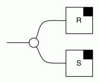
This is not the case for the number system from Episode 26. In fact, the three additional elements ∞, ⊥, ⊤ do show up in calculations. The cool thing is that they are not a sinkhole like NaN: you don’t need to panic if you get, say, a ⊥ in one of your calculations. It’s possible that things will finish well. This episode is entirely devoted to one example: inverting matrices.

We will need a few definitions.

An n×m matrix A is said to be invertible when there exists an m×n matrix B, such that when you compose in either direction, you get the identity. In diagrams:

If such a B exists, we sometimes write A^-1 = B. Many matrices are not invertible. One property of those that are is that m=n, that is, invertible matrices are all square; the number of rows is equal to the number of columns.

Actually, it’s like this in most PROPs – you can usually only invert things where the left and the right boundaries have the same size. A useful intuition to keep in mind is that something can only be invertible if it can be undone. And since wires carry information, we can’t just throw one away or add a new one and expect to be able to undo it.

Back to definitions. We will say that an n×m matrix A is injective, or mono, when the following is true.

The backwards facing A is none other than the mirror image symmetry † that we discussed in Episode 27.

The above definition probably seems a bit strange. In most ordinary linear algebra textbooks, the defining property of an injective n×m matrix is that it takes  different m-vectors to different n-vectors: that is, it is injective as a function. This is actually an equivalent formulation, but we don’t think about matrices as functions on this blog.

One interesting property of mono matrices is that they are left-cancellable: that is, given two equal-sized matrices B, C for which AB and AC is defined, if AB=AC then B=C. In fact, this is true when B and C are linear relations. Diagrammatically:

implies that

Here B and C are linear relations, i.e. arbitrary diagrams in IH. This of course includes the case where B and C are matrices.

Actually injectivity and left-cancellability are also equivalent, i.e. assuming one, you can prove the other. I’ll leave the proofs as an exercise but I’ll give you a hint: it’s handy to use the fact, stated in Episode 27, that for any linear relation A, A^† is its weak inverse.

The bizarro of injective is surjective. We will also use the word epi. Thus, an n×m matrix is surjective when the following is true:

Just as mono matrices are left-cancellable, epi matrices are right-cancellable; given B and C such that BA and CA make sense, if BA=CA then B=C. In terms of ordinary linear algebra, surjective matrices are those that are surjective as functions; for every n-vector b, there exists an m-vector a such that Aa=b.

There is one final observation that we will need later: any invertible matrix is both injective and surjective. To keep things moving along, I’ll also leave the proof of this as an exercise.

Let’s now prove a classic result of linear algebra. It refers to kernels and images, which are linear subspaces that we discussed in the last episode.

Kernel and Image Lemma. Suppose that A is an m×n matrix. Then:

1. A is injective exactly when it has a null kernel
2. A is surjective exactly when it has a full image.

Proof. Properties 1 and 2 are mutually bizarro, so it’s enough to prove just one. We will do 1.

Suppose that A is injective. Then:

Which means that A has a null kernel.

Suppose now that A has a null kernel; we want to show that it must be injective.

That’s it, we’re done, QED.

The following lemma is very useful because it gives us some useful graphical intuition about invertible matrices.

Invertible Matrix Lemma

Suppose that A is a square matrix of size m. Then the following are equivalent

1. A has inverse B
2. There exists matrix B such

Proof. Let’s first show that 1 implies 2. Assuming 1, Suppose that A has inverse B. Since A is invertible, we know that A is injective. So we have the following:

Which gives us 2. In the first step, we used the assumption that B is the inverse of A, and in the second step we used the fact that A is injective.

We still need to show that 2 implies 1. So, supposing that A is equal to some matrix B heading in the opposite direction, we need to show that B is the inverse of A. To do that, it’s useful to show that A must be injective. Here we can use our Kernel and Image Lemma.

So, by the kernel lemma, A is injective. We can now use this to show that A followed by B is identity.

To show that B followed by A is also identity, we can do the bizarro thing, first showing that B is surjective.

Our aim is to obtain a formula for the inverse of a matrix, if it exists. The starting point is an arbitrary 2×2 matrix, so something like this:

If an inverse exists, then we know it’s also going to be a 2×2 matrix:

The tricky part is, how can we calculate a’, b’, c’ and d’, knowing a, b, c and d? If you remember your linear algebra, maybe you’re thinking determinants and adjugate matrices. We will bypass all that and draw some pictures instead.

Let’s start by using our Invertible Matrix Lemma. As diagrams in IH, we have:

Now adding a matrix to -1 times itself gives us the zero matrix. Using this trivial observation, we get the following rather complicated looking equation:

We can extract the formula for each of a’, b’, c’ and d’ by plugging up some of the dangling wires in the above equation. Let’s work through the procedure for a’.

The first step is to plug a zero and a discard at the right places in both sides, like so:

Doing that, we get the first equality below.

The second equality follows from the bone equation of bimonoids.

So far so good: but now we can drastically simplify the left hand side. Essentially, we’ve plugged a white unit into a black comultiplication, and vice versa; usually when that happens, there is mass destruction. I’ll leave the graphical derivation to you. After you’ve killed off most of the diagram, the left hand side ends up looking like this:

The nice thing is that now a’ is the only entry from the inverse matrix that’s left. And we already know that the diagram above is equal to zero, i.e.

So we are in the situation where a’ plus -1 times some mess is equal to 0; thus:

This is starting to look like a formula. We can untangle the still somewhat messy right hand side above. The result is:

In terms of a bona-fide, old-fashioned syntactic formula—if you’re into that kind of thing—this translates to:

Note that I did not go further in simplifying the denominator because d might be zero, and in that case, multiplication may not be commutative. Relax; to evaluate the formula for specific numbers, we can use our addition and multiplication tables from Episode 26.

There is nothing special about a’. We adapt our procedure by plugging up the other combinations of wires and obtain formulas for b’, c’ and d’. All together:

I find it quite cute how a, b, c and d permute in each of the formulas. And no determinants, nor adjugates in sight!

Let’s do a worked example, calculating the inverse of the matrix:

Referring to the formula for the inverse, we have d=0, so we will divide by zero when calculating a’. For that, we can refer to the multiplication and addition tables from Episode 26. Here’s the calculation:

The other calculations don’t involve any funny stuff — we end up with

I promised you an example where the extended rational algebra of Episode 26 can be useful. And while inverting 2×2 matrices is not going to set the world alight, I hope that this is a hint that there is something interesting going on!

By the way, the formula that we derived for inverting 2×2 matrices generalises to arbitrary square matrices. I don’t have the space for this in this episode, but if there’s interest I can come back to this topic. Let me know.

Not writing is like not going to the gym (which, coincidentally, I’m also guilty of). I mean that once you start not writing, it’s difficult to get back into it. “I’ll do some writing next weekend” – you tell yourself. Before you know it, half a year has passed. Same with (not) going to the gym. I’m still working on that.

Having said that, it’s been a very busy half a year. In addition to teaching,  I visited Paris—and more specifically, Jean Krivine—for a month. I love Paris; I spent a six-month postdoc there in 2005 and it was fantastic to be back in the 13^e arrondissement.

Apart from enjoying the city, it was a really productive visit and I learned a lot. Jean is currently working on a graphical high-level programming language for biologists, which shares many features with the kind of string diagrams that this blog is obsessed with.

Amongst other things, Jean told me about a family of string-diagrammatic calculi for logic, developed by the famous 19th century American logician C.S. Peirce (pronounced “purse”; it’s Dutch, apparently). Jean uses some of Peirce’s ideas for his programming language. Peirce’s systems are called existential graphs and have a fascinating history.  While Peirce considered them his most important scientific achievement, they remained unpublished in his lifetime; I guess due to a lack of typesetting technology for diagrams, but maybe also due to the fact that his ideas were so revolutionary that they were about 100 years before their time. In fact, Peirce’s diagrams came before the standard syntactic way of writing logic, with all the upside down As and backwards Es that logicians are so fond of. But his work was forgotten and were rediscovered only in the 1960s. They are still a topic of research.

Existential graphs really blew me away. I plan to understand them properly over the next few months, and maybe I will write about them more seriously one day. For now, if you’re interested in reading further, the PhD thesis of Frithjof Dau seems like a great resource.

This weekend I will be in Porto for the HDRA workshop, and the weekend after that I’m flying to New York for the LiCS conference. It’s going to be a busy summer, but I will try to work more regularly on the blog from now on.

Continue reading with Episode 30 – The essence of graphical linear algebra.