28. Subspaces, diagrammatically

There are two common ways to interpret the information represented by a matrix. Roughly speaking, it boils down to whether—when looking at a grid of numbers—you choose to see a list of columns, or a list of rows. The two interpretations are symmetric, and this is nicely captured by this blog’s obsession, the graphical syntax. And as we will see, the two ways of looking at matrices will lead us to two different, symmetric ways of understanding linear subspaces.


Consider an m×n matrix A, drawn with our graphical sugar for matrices as a gadget with n wires entering on the left and m wires exiting on the right, like so:

matrix

A can be viewed as consisting of n column vectors c1, c2, …, c. Each of the c‘s is individually a m×1 matrix, so it has one wire entering on the left and m wires existing on the right. We can then wire up A, emphasising the column vectors, like so:columns

Alternatively, we can view the same matrix A as consisting or of m row vectors r1, r2, …, rn, with each having n wires on the left and one wire exiting on the right. This leads to drawing A like this:rows

Even though in both cases we are talking about the same matrix—the same raw data—it turns out that the two different points of view lead to two quite different interpretations.


Let’s work through a concrete example. Consider the matrix

matex

which has no particular significance; I just pulled it out of a hat, so to speak. But it’s usually a good idea to have a particular, concrete object to work with, and this one does the job.

Emphasising the columns, it can be drawn like this:

colsex

Or we can focus on the rows, as shown below.

rowsex


Viewing a matrix as a list of columns leads to the first interpretation of what a matrix means: a recipe for of transforming n vectors—that is, columns of of n numbers—into m vectors, i.e. columns of m numbers.

Indeed, let’s take another look at A drawn in the way that emphasises its columns.

columns

We can imagine the n dangling wires on the left as being n different inputs. Now each ci takes an input number and produces a column of m numbers. At the end, the n columns, each of size m, are simply added up.

Let’s work through an example to see how this works, using the concrete matrix from before.

columnsex

Here, our input vector consists of 51 and -2. Each input results in two outputs, according to the recipe within each column block. They are then added up, e.g. 5+(-1)+(-2)=2 in the first output. Using the standard linear algebra jargon, we have produced a linear combination of the column vectors:

linearcomb

In our worked example above we took one particular, quite arbitrary choice of inputs: 5, 1 and -2. This leads to a natural question: exactly which vectors can be produced by this circuit, supposing that we are free to choose any inputs whatsoever.

In the example above, it turns out that all outputs can be produced by picking the appropriate inputs. But this is not always going to be the case; for example, if all the columns consist of only zeros then clearly only the zero output is possible.

The general question is, then, the following: given column vectors c1c2, …, cn, which m vectors can be written as a linear combination

α1c1 +  α2c2 + … + αncn?


How can we express this idea in our graphical language?

It turns out that the idea of considering all possible inputs is simple to describe. It is also quite intuitive. First, let’s return to our venerable discard generator.

discard

Recall that our intuition, backed by the functional semantics, is that this simply discards any number given to it. With matrices, we usually like to think of numbers flowing from left to right. So what are we to make of discard’s mirror image?

generate

Well, if the discard can throw away any number, then a nice way to think about its mirror image is that it can generate any number. So, to get back to our original question, we can talk about the linear subspace of Qm generated by the matrix A by simply considering all the possible inputs to each column. Like so.

range

The diagram now represents the subspace that consists of all the linear combinations α1c1 +  α2c2 + … + αncn of A‘s column vectors, where each α is a fraction. More precisely—as we have discussed in the last episode—the diagram gives us a linear relation of type Q⇸ Qm, which we can (since Q0 contains only one element) then simply think of as a subspace of Qm.

This subspace is quite famous and has several names; it’s variously called the image, range, or column space of A, or the span of c1, c2, …, cn. And, using our usual syntactic sugar, we can simply write it as:

rangesugar


I claimed above that our example matrix can produce any pair of outputs. Let’s do the calculation to make sure: it’s a nice little exercise in diagrammatic reasoning.

imageex

The image is thus the entire space Q2, so for any pair of fractions p, q we can indeed find inputs u,v,w such that

Auvw


Viewing a matrix as a collection of rows leads to another popular interpretation of the information that a matrix represents: a list of equations that constrain the inputs. Let me explain.

Drawing A in a way that emphasises the rows, we can think of each ri as encoding a linear combination of the inputs.

rows

For example, going back to our original matrix, let’s label the inputs with variables x, y and z.

rowsex2

So the rows tell us how to combine the various inputs to form the outputs: for example, the first row gives us x-y+z and the second 2y+z.

Here, the natural question is to think of the rows as homogenous equations, and consider the set of solutions, those concrete choices of x, y and z that satisfy them. Homogenous, by the way, means simply that we append = 0 to each linear combination of variables.

So for our running example, we could consider the collection of all the inputs constrained so that they satisfy the two equations:

x-y+z = 0                  ①             

2y+z = 0                  ②


We can also represent this graphically. When we emphasised the columns, we introduced a new intuition for the mirror image of discard. This time we are focussing on the rows, and so, not surprisingly, we will introduce a new intuition for the mirror image of the zero generator.

Recall that the zero generator, in the original left-to-right functional interpretation, simply outputs 0.

zero.gif

So how are we to think of it’s mirror image?

constrainThe answer is that it’s a constraint: it only accepts 0!

Using this insight, the solution set of the list of homogenous linear equations given to us by the rows of the matrix A is graphically represented as:

kernel

or using our usual sugar:

kernelsugar

This is a linear relation of type QnQ0, so for the same reasons as before, it’s pretty much the same thing as a linear subspace of Qn. This subspace is also very important in linear algebra, and is variously called the kernel, or the nullspace of A.


Let’s do a calculation that will give us more information about the kernel of our long running example matrix. The calculation is a bit longer than before, but the details are not so important at this stage.

kernelcalc

In the derivation we used the Spider theorem from Episode 23.

Here’s the interesting thing about the calculation: we started with a diagram in which we were thinking of the “flow” as going from left to right, where our inputs had to satisfy some equations. We ended up with a diagram which is easier to understand as going from right to left. Indeed, it’s an example of the kind of subspace that we got by focussing on the columns; it is:

N.gif

where N is the matrix

Bmat.gif

In other words, the kernel of M is the same linear subspace as the image of N. This tells us that everything in the kernel is of the form

kerneldesc

where α is some fraction. So the solutions of the system of equations  and  are x = 3α, y = α, z = -2α.


We have seen that some descriptions of a linear relation can be read “from left to right” and others “from right to left”. Indeed, we have just seen an example of a linear relation that had two descriptions:

spaceeq.gif

So what is really going on here? It turns out that we can think in two ways about every linear relation.

  1. Every linear relation can be seen as “being generated”, in the way we described the image subspace.

rangesugar2. Every linear relation can be thought of as consisting of the solutions of homogenous equations, of inputs “being constrained”, the way we described the kernel subspace.kernelsugar

Let’s be more precise about this. We will start by considering the first of the two situations, the “being generated” case.

The proof of IH ≅ LinRel—which we haven’t seen yet but we will go through in due course—has one important consequence: for every linear relation R: m⇸n we can find an m×p matrix A and n×p matrix B such that

spanform

If we have such matrices A, B then we will say that they are a span form of R. Span forms allow us to think of R as being generated. In fact,

rangesugaris in span form, since

ndiscardis the graphical representation of the unique 0×n matrix.

The proof of IH ≅ LinRel also gives us the “being constrained” case, which is pleasingly symmetric. For every linear relation R:m⇸n, we can, respectively, find q×m and q×n matrices C and D such that

cospanform

This is called a cospan form of R. Cospan forms capture the idea that a linear relation can be thought of as the solution set of a bunch of homogenous equations. An example is the kernel of a matrix A

kernelsugar

since

zerom

is the unique m×0 matrix.

One little quirk of history is that the traditional way of doing linear algebra focusses very heavily on the span view, and almost totally ignores the cospan view. One takes a space and finds a basis, one talks about its dimension, etc. But the cospan view is just as expressive, given the symmetries of graphical linear algebra. So, it’s entirely possible that Martian linear algebra has been developed in a way that prioritised the cospan view of linear subspaces. It’s fun figuring out the details, and we will do some of this in the next episode!


I’m having a very heavy start to 2016: originally I was planning to publish this episode in early January, and it’s now early February. The highlight of the month was a trip to Oxford on Friday January 8. I was there to examine a thesis entitled “!-Logic: First-Order Reasoning for Families of Non-Commutative String Diagrams” of (the now Dr.) David Quick, supervised by Aleks Kissinger. I liked the thesis very much: it’s about a logic for string diagrams, much like the ones on this blog. David’s logic supports reasoning about whole families of diagrams, including supporting sophisticated inductive arguments; much more sophisticated and powerful than the kind of induction that we have been using on the blog. I will have to write about it at some point in the future.

I arrived in Oxford quite early, and it was a really beautiful morning. On my walk from the train station to the computer science department I got the urge to take a photo.

12417944_10153936526981383_3321537427747874569_n.jpg

The next Friday, January 15, I was in Cambridge to give a talk. That trip was also a lot of fun, and I got the chance to catch up with some old pals. The evening was very pleasant, and I decided to walk from the computer science department to the train station. On the way I took this photo:

11237564_10153952837936383_628595388964310973_n

I later noticed—and I promise, as much as it looks like it was, this wasn’t planned!—that the photos themselves are quite symmetric: compare the relationship of water to land. Since we spend a lot of time talking about symmetry on this blog, I think it’s somehow appropriate.

Continue reading with Episode 29 – Dividing by zero to invert matrices.


Advertisement

27. Linear Relations

In the last two episodes we focussed on fairly simple diagrams in IH: those with just one dangling wire on each end. In this episode we expand our horizons and consider arbitrary diagrams. It’s time to return to linear algebra. We will also revisit division by zero from a different, but equivalent, point of view.

We’ve known since Episode 10 how to handle matrices diagrammatically, and since our expanded graphical language can handle fractions, we can put the two together and draw matrices of fractions. The algebra works as expected: if we restrict our attention to these matrices, composition is matrix multiplication, and the monoidal product of two matrices is their direct sum. Here’s a reminder of how to draw, say, the following matrix

firstmat

exmatfrac

But we can do much stranger things. Since we have the mirror image operation  in our arsenal, we can consider matrices going backwards. We don’t have any traditional notation for this: how could you write a matrix that “goes backwards”?  But here’s an example in the language of diagrams, if

secondmat

Then we have can draw the diagram for B going from right to left.

exback

Matrices and backwards matrices are not the full story because diagrams can get more complicated. In general, diagrams from m to k will be quite strange beasts: imagine a zig-zag of matrices going back and forth. It’s as if we took our Lego and got confused about what are the studs and what are the holes. Everything goes.


Let’s clear up the mystery. We know that the sub theories B and H are isomorphic to, respectively, the props Mat of matrices of natural numbers  and MatZ of integer matrices. Knowing this helped us to understand the diagrams in those theories, and what they were capable of expressing.

So, without further ado, it’s time to meet the linear algebraic prop LinRel that hides behind the equations of graphical linear algebra. Coincidently it’s my favourite category, so please forgive me if I sound a bit too much like a fanboy in the following. Before we start, we need some notation: in the following, the bold letter Q stands for the set of fractions, aka the rational numbers.

The arrows from m to n in LinRel are linear relations from Qm to Qn. Roughly speaking, LinRel is what happens when you combine matrices and relations. The result is truly delightful; it is much more than the sum of its parts. You will see what I mean.

Before I explain what linear relations are in more detail, let me first say that it’s a huge mystery that the concept of linear relation does not seem to be particularly standard or well-known: there is not even a wikipedia page at the time of writing this episode! Since there’s an informative wikipedia page about, say, Cletus from the Simpsons, this is a bit offensive. Maybe it’s because of a human preference for functional thinking, at the expense of relations? We discussed that a bit in Episode 20.

So what is a linear relation exactly?

First, a linear relation of type Qm ⇸ Qn is a relation, so a subset of the cartesian product Qm × Qn. De-jargonifying, this means that it’s a collection of pairs, with each consisting of an m-tuple and an n-tuple of fractions. For example, the linear relation for the addition generator—which we have already discussed informally in Episode 22—is the relation of type QQ that consists of all pairs

addrel

where r and s are fractions. We have thus finally demystified what the enigmatic universe of numbers Num is: for now Num = Q, our numbers are fractions.

We still need to account for the word linear in linear relations. Said succinctly, to be linear, a relation  R: Qm ⇸ Qn must be a linear subspace of Qm × Qn, considered as a Q vector space. If you don’t know what those words means, let me explain.

First, R must contain the pair of zero columns.

zero

R must also satisfy two additional properties.The first is that it must be closed under pointwise addition. This scary sounding condition is actually very simple: if R contains pairs

ab

and

cd

then it also must contain the pair obtained by summing the individual numbers:

abpluscdIt takes a lot of space to write all those columns, so let’s introduce a common notational shorthand: we will write a for the a-column (or column vector), b for the b-column and so forth. When we write a+c we mean that a and c are columns of the same size and a+c consists of a1+c1, a2+c2 and so on until am+cm. So—using our new shorthand notation—for R to be closed under pointwise addition, whenever (ab) and (cd) are both in R then also

(a, c) + (b, d)  :=  (a+c, b+d)

must be in R.

The second property of linear relations is that they must be closed under scalar multiplication. This means that whenever

ab

is in R then also

kab

must be a member, where k is any fraction. We can also do say with the shorthand notation: given a vector a and fraction k, we will write ka for the vector with entries ka1, ka2, …, kam. So, being closed under scalar multiplication simply means that if a is in, then ka must also be in.


Composition in LinRel works just like it does in Rel, so composing R: Qm ⇸ Qn and S: Qn ⇸ Qp gives R;S : Qm ⇸ Qp with elements (x, z) precisely those for which we can find a y such that (x, y) is in R and (y, z) is in S.

I claim that LinRel is a prop. To be sure, we need to do some things that may not be immediately obvious:

  1. verify that the identity relation is a linear relation,
  2. check that composing two linear relations results in a linear relation, and
  3. say what the symmetries are and make sure that they work as expected.

The first one is easy, try it!

For point 2, we need to show that if R: Qm ⇸ Qn and S: Qn ⇸ Qp are linear relations then so is R;S.

Let’s prove closure under pointwise addition: suppose that (x1z1) and (x2z2) are in R;S. We need to show that (x1+x2, z1+z2) is also in R;S. Using the definition of relational composition, there exist y1, y2 such that (x1y1) and (x2y2) are both in R and (y1, z1) and (y2z2) both in S. Since R and S are linear relations, they are both closed under pointwise addition, so we can conclude that (x1+x2, y1+y2) is in R and (y1+y2, z1+z2) is in S. It thus follows that (x1+x2z1+z2) is indeed in R;S. I’ll leave you to check that it’s closed under scalar multiplication, the argument is very similar.

For point 3, for now I’ll just tell you what the relation for the twist 2 → 2 is and hope that it gives you the general idea. The twist in LinRel is the smallest linear relation that contains the elements

twist

Since we need to close under addition and scalar multiplication, elements in this relation will look like

twistgen

where k and l are fractions.


We have already discussed the relational semantics of the generators in Episodes 22, 23 and 24 and verified that the equations make sense, relationally speaking. It is not difficult to check that each of the relations is linear. Long story short, this assignment of relations to generators defines a homomorphism of props

IHLinRel.

As we will eventually prove, this is an isomorphism; it is both full and faithful.

The proof of IH ≅ LinRel is quite a bit more involved than the proof BMat and H ≅ MatZ. We will eventually go through it in detail—apart from following our principle of not handwaving, the proof is quite informative. But for now, LinRel and its diagrammatic presentation IH are perfect playgrounds for linear algebra and that’s what we will concentrate on over the next few episodes.


In the last episode we discussed how (1, 1) diagrams allowed us to divide by zero. By looking at the corresponding situation in LinRel, we can shed some more light on this curiosity. So let’s take a look at linear relations  Q: since IHLinRel these are in 1-1 correspondence with (1, 1) diagrams.  We can plot linear relations of this type using conventional graphical notation, thinking of the domain as the horizontal x axis and the codomain as the vertical y axis.

Since every linear relation must contain the pair that consists of zero columns, every plot will contain the point (0,0). In fact, the singleton {(0,0)} is itself a linear relation: clearly it satisfies the two required properties. Here’s its plot.

bot

The diagram for this linear relation is

botdiag

which we dubbed ⊥ in the last episode. Next up, the entire set Q×Q is a linear relation. Here we colour the entire plane red. Sorry for the eye burn.

top

The corresponding diagram is

topdiag

which we were calling  last time. These two linear relations give some justification for the names ⊥ (bottom) and ⊤ (top), since the former is—set theoretically speaking—the smallest linear relation of this type, and the latter is the largest.

The other linear relations are all lines through the origin. So, for example, the plot for the identity diagram

iddiagis the line with slope 1.

id

All the fractions arise like this. For example, the line for the fraction 1/2,  diagrammatically

minhalfdiag

is the line with slope 1/2

minhalf

You get the idea for the other fractions.

There are two lines that represent interesting corner cases. The first is the line for 0

zerodiagwhich is the line with zero slope, that is, the x-axis.

zeroline

Finally, there’s the line with “infinite” slope, the y-axis.

infline

which is the plot for

infdiag

that we called  in the last episode.

If we think relationally, then the operations x+y, x×y and 1/x are all easy to define, and are total on the set of linear relations  Q. Multiplication is simply relational composition, and 1/x is the opposite relation x. Finally, addition can be defined set theoretically as

x + y = { (a, c) |  there exist (a, b1) in x and (a, b2) in y such that b1+b2 = c }.

The above definition simply mimics the sum operation, as we have been doing with diagrams. So we could reconstruct the addition and multiplication tables from the last episode by working directly with linear relations.

Identifying numbers with lines through the origin is an old idea. It is one way to understand projective arithmetic. What is not so well-known is that we can define the arithmetic operations directly on the underlying linear relations, and moreover, throwing ⊤ and ⊥ into the mix makes the operations defined everywhere, with no need for dividebyzerophobia. If you have seen this done somewhere else, please let me know!


Here’s one very cool fact about LinRel, and it concerns the mirror image symmetry . Remember that if R is a relation then R is the opposite relation: (ba) is in R exactly when (ab) is in R. In the last episode we saw that for any (1,1) diagram d we have

d;d;d = d.

It turns out that this works for arbitrary linear relations. Thus R is always the weak inverse of R. This is something that will be very useful for us in the future. Let’s prove it.

Suppose that D is some linear relation. Since D;D;D and D are both sets (of pairs), to show that they are equal it’s enough to show that each is a subset of the other. It is easy to show that every element of D must be an element of D;D;D, since, taking (a,b) in D, the chain of elements (a,b), (b,a), and (a,b) proves that (a,b) is in D;D;D.

We just need to show that the opposite inclusion also holds. So suppose that (a, d) is in D;D;D. By definition, there are bc such that (ab) is in D, (b, c) is in D and (cd) is in D. And since (bc) is in D, (cb) is in D.

Now, using the fact that D is a linear relation that contains (ab), (cb) and (cd), we have that

(a, b)-(c, b)+(c, d) = (ac+c, bb+d) = (a, d)

is in D.

The fact that D;D;D is not larger than D is one thing that’s special about linear relations: it is not true for ordinary relations! For example, think about what happens to this relation 2 ⇸ 2:

weakcounter


Today is Boxing Day, so this is a Christmas special episode of the blog. The next one will probably arrive in January, so let me take this opportunity to wish everyone a fantastic

2016


Continue reading with Episode 28 – Subspaces, diagrammatically.


26. Keep Calm and Divide by Zero

The fear of dividing by zero is a common affliction. I caught it at school when trying to get my head around this well-known “proof” of 1 = 2:

  1. suppose that a = b
  2. then a2 = ab
  3. subtracting b2 from both sides gives us a2 – b2 = ab – b2
  4. factorising gives (a + b)(a-b) = b(a-b)
  5. dividing both sides by a-b gives a+b = b
  6. But also a+b = b+b = 2b, so 2b = b. Dividing by b gives 2 = 1.

The problem is in step 5, in which both sides of the equation are divided by zero: helpfully, this article with a similar wrong proof explains that you cannot ever do that.

Looking at the available evidence in popular culture, interest in dividebyzerophobia is prevalent: for example, this Numberphile video has over 2 million views. Even Siri has something amusing to say.

So I was understandably very nervous when I first realised that graphical linear algebra lets you divide by zero. I double checked everything: something must have gone seriously wrong.

Let me explain.

In the last episode we saw that ordinary fractions v/w (where w≠0) can be represented as the sugar:

sugardef

We then discovered that the usual rules for doing arithmetic with fractions follow from the equations of our algebraic system:

addition

multiplication

The derivations made use of the fact that q and s are not zero.

So far so good, but there’s an important difference between fractions and our diagrams. Fractions are inherently asymmetric: the numerator is allowed to be zero, but the denominator is not. On the other hand—as we saw two episodes ago—the generators and equations of graphical linear algebra are symmetric.

So, since by definition we haveoneandzero

if we can draw the diagram for 0/1, then there’s nothing stopping us from drawing the diagram for 1/0:

onedividedbyzero

But we are never allowed to do this, right?

Stay calm and take a deep breath: dividebyzerophobia is an irrational fear, caused by a deficiency of the fraction notation that we all grew up with. I no longer suffer from it and, with the right dosage of graphical linear algebra, neither will you.


As we have seen, all fractions are diagrams with one dangling wire on the left and one on the right. But—as we just discovered—not all diagrams of this type are legal fractions. In fact, there are precisely three that fail to be of the right form, and they all involve dividing by zero in some way. Let’s give them names:

extraelms

It makes sense to choose ∞, the symbol for infinity, as the name for the 1/0 diagram: for example 1/x diverges to positive or negative infinity as x approaches zero. And positive and negative infinity are one and the same in projective arithmetic.

We will come back to projective arithmetic in more detail in the next episode. For now, let’s verify whether our diagrams indeed tell us that positive and negative infinities are equal.

posneginft

The remaining two elements,  and ⊥, are two ways of resolving what we might mean by 0/0, which is ambiguous. This ambiguity does not exist when talking about ordinary fractions: if w is nonzero, the following two diagrams are equal, using the fact that nonzero sugars commute with sugars heading in the opposite direction. We showed that in the last episode.

equalfractions

So both of these diagrams represent the fraction v/w. But when v=w=0, the two diagrams are different: the first is , the second .


I’ve coloured ∞, ⊤ and ⊥ differently from our usual sugars, because, as we will see, they don’t behave quite as well as ordinary fractions. Nevertheless, we can try to do arithmetic with them as we did with fractions.

For example, what happens if we take some (legal) fraction p/q and add it to ?

fracplusinfty

We seem to get stuck at this point because we don’t have any equation that tells us what happens when we plug the (wrong way) zero generator into a copy. It turns out that:

dagger

Here’s a derivation:.

lemma

Using what we know about symmetry in graphical linear algebra, we can immediately state the bizarro version, which is

ddagger

Continuing our calculation , we get

fracplusinfty2

So, given any fraction p/q we have that p/q + ∞ = ∞. In fact, using (†) and (‡), we can also show that  ∞ + ∞ = ∞,  ⊤ + ∞ = ∞ and ⊥ + ∞ = ∞. So anything plus infinity is infinity.


In the fifth line of the above calculation we used a property we have not yet proved, that whenever w ≠ 0, the w can come out of a discard. This property is related to one from the last episode: nonzero sugars can go the wrong way over copy. Here’s a reminder of what this means, together with its bizarro version:

wrongway

To keep a clear conscience, let’s prove the new property. Its bizarro version, which says that the zero generator can swallow nonzero sugars, will also come in handy in proofs.

wrongwayunits

Using the usual symmetry argument, it’s enough to prove one.

proofwrongwayunit

Also, since we didn’t do it earlier, this seems a good time to check whether 0/w is actually the same as 0. In the second step we use our new fact about the zero generator and nonzero integer sugars.

zerofrac


We may as well fill out the full addition table, which takes account of all possible ways that (1,1) diagrams can be added. In the table below I separated 0 from the nonzero fractions, where both the numerator and the denominator are not zero.

Remember that our diagrammatic addition is commutative, so we don’t need to fill the table below the diagonal.

+ 0 r/s
0 0 r/s
p/q sp+qr/qs

Perhaps the most mysterious equation in this table is ⊤ + ⊥ = ∞. It’s very simple to justify:

topplusbot

Multiplication is a bit more hairy, because although it is commutative on ordinary fractions—as we saw in the last episode—it is not always so when we consider the expanded system with the additional three elements. This means that now we need to fill in the entire table.

× 0 r/s
0 0 0 0
p/q 0 pr/qs
0 0

There are some interesting symmetries in the table. And we can resolve the old philosophical conundrum about what happens when we multiply infinity by zero! In graphical linear algebra it turns out that 0 × ∞ = ⊥ and ∞ × 0 = ⊤.


What do we really mean by “dividing by zero”? As Siri says, it does not make much sense to divide cookies amongst zero friends; even when the Cookie Monster is happy, you are still sad.

Graphical linear algebra comes with the mirror image symmetry. We will use the dagger () superscript to mean mirror image. So if d is a diagram of type (m,n) then its mirror image d is a diagram of type (n,m). Clearly, no matter what the d, we always have d†† = d.

When d is a nonzero fraction sugar, then it turns out that d† is the multiplicative inverse of d: this means that d ; d† = d†; d = 1. It’s an easy derivation:

multinv

When d is 0 or  then this is no longer the case, as can be seen from the multiplication table. For example 0 ; 0†  =  0 ; ∞  =  ∞ × 0  =  ⊤ and 0† ; 0 = 0 × ∞ = ⊥.

Since does not always mean multiplicative inverse, what are some properties that it does satisfy for all (1,1) diagrams? Here is one: d and d are the weak inverse of each other.

d ; d ; d = d

d ; d ; d = d

I’ll leave this as a simple exercise. It will be great as the first step in your dividebyzerophobia treatment programme. For nonzero fractions, the equations follow from the fact that gives us the multiplicative inverse. To treat the other cases, you will only have to do four calculations, because  = ⊤ and  = ⊥.

The mirror image symmetry will be very useful when we talk about inverting matrices in graphical linear algebra. I’m thinking of bringing some of this material forward—maybe already to the next episode—because it is a nice example of how dividing by zero can actually be useful in calculations.


Although it was fun to fill in the addition and the multiplication tables, there are good reasons not to give  and  the same status as we give to the numbers (naturals, integers, fractions) that we have seen so far, and others (reals) that we will talk about in the future. This is why we have been colouring their sugars differently.

I don’t plan to get bogged down in a philosophical discussion about “what is a number?” (Episode 17 did not seem to go down too well) but there are a number of useful properties that “numbers” ought to satisfy in graphical linear algebra. For one, the bizarro of a number should be itself. This works for ∞, but ⊤ and ⊥ are the bizarro of each other.

It is also very useful to know that numbers, whatever they are, satisfy the following:

usual

We know from earlier episodes that they hold for the natural numbers and for the integers. Given what we now know about nonzero sugars going “the wrong way” over copy and addition, and into discard and zero, it is follows that they hold for fractions as well. So, the a in the above equations can be any legal fraction.

These properties allow us, amongst other things, to prove that multiplication distributes over addition. But all three of  and ⊥ fail some of these four tests. For example, we have:

inftyfailure

And these two diagrams cannot be shown equal in our theory. For now, you could think about the underlying relations, but we will get more precise about characterising diagram equality in the next episode.

So—long story short—while we will not think of them as numbers per se, we will not panic when we see and  popping up in calculations. They are all perfectly harmless.


In algebra, the notion of a set of elements with addition and multiplication, where multiplication is commutative and distributes over addition is called a commutative ring. If all nonzero elements also have a multiplicative inverse, the resulting structure is called a field. The rational numbers (i.e. fractions) and the real numbers are two examples.

Fields are a little bit peculiar from an algebraic perspective, because the operation of taking multiplicative inverse is partial0-1 is left undefined. Having partially defined operations complicates things.

One classic way of addressing this defect is projective arithmetic, which we will see in more detail in the next episode. There 1/0 makes sense, but 0/0 is still typically left undefined. Recently, inspired by projective arithmetic, Youtube legend Norman Wildberger proposed to hack fraction notation so that 0 is allowed in the denominator: you can check out some videos starting from this one. I have not yet had the time to understand the details, but it seems that you have two new elements that correspond to 1/0 and 0/0; the latter seems to be our  but there is no .

There are some other algebraic systems that go the whole hog and make all operations defined everywhere. Two that I’ve come across are wheels and meadows. If there is interest, I can write more about these; let me know in the comments.

There is one fundamental difference between the above approaches and arithmetic in graphical linear algebra. There, existing notation (e.g. addition, multiplication, fraction notation) and associated equational theories were extended in some way to make sense of dividing by zero. In graphical linear algebra, addition is not even a primitive operation, or at least it’s not primitive in the same sense. So instead of setting out to make sense of 1/0, we discovered that it was already happening, in a similar way to how we discovered the natural numbers lurking in the theory B of bimonoids.


I was in Edinburgh for a couple of days last week. I left Southampton on a cold, dark and wet morning and arrived in a Scotland bathed in glorious sunshine.

I was there as the external examiner for the PhD defence of Ricardo Honorato-Zimmer, a student of Vincent Danos. It was great to have the chance to catch up with Vincent. He is one of the few scientists I know who is a true polymath—his background is the French school of logic, and his early contributions to the proof theory of linear logic are pretty famous. Around ten years ago, Vincent became interested in stochastic formalisms and graph rewriting, and together with a number of people he developed the Kappa language for modelling protein interaction networks. Vincent’s group is now full of chemists, biologists, mathematical physicists, mathematicians and computer scientists who all manage to communicate (this is far from easy in my experience!) and moreover come up with real advances. Academic politicians like to throw around the term “multi-disciplinary research”, but often the reality behind the buzzword is somewhat underwhelming. It’s always amazing to see the real thing in action.

The day after the defence I gave a short talk about graphical linear algebra at the LFCS seminar. Afterwards I met Kevin Dunne, who is doing a PhD with Ross Duncan at the University of Strathclyde in Glasgow. Kevin told me his idea about how to develop the theory of eigenvalues and eigenvectors with graphical linear algebra: it sounded fantastic and I’m really looking forward to figuring out the details. I also met Nick Behr, who is a mathematical physicist working with Vincent. He told me about the Umbral calculus, used to reason about formal power series, and we tried to figure out the relationship with some related techniques that Filippo, Fabio and I developed using graphical linear algebra. He will visit Southampton for a few days in January; it’s going to be exciting!

I had to come back to Southampton not long after my talk. This time, I experienced some more common Edinburgh weather: I walked from the computer science department to Waverley station in rain and gale force winds. The locals seemed undisturbed.

Continue reading with Episode 27 – Linear Relations.


25. Fractions, diagrammatically

I’ve been looking forward to this moment for some time. Now that we’ve gone through all of the equations of graphical linear algebra, it’s time to have some fun. In this episode we look at how fractions are represented in the graphical notation, derive the usual rules of fraction arithmetic, and go through a very early example of an algorithm that produces fractions: Fibonacci’s procedure for division by composite numbers.

We will concentrate on diagrams with two dangling wires: one on the left and one on the right. In previous episodes we have seen that these diagrams have a tight relationship with various kinds of numbers. For example, in the theory of bimonoids, a sub-theory of graphical linear algebra, they were in 1-1 correspondence with the natural numbers. When we added the antipode, extending the theory, we got the integers.  Since then, we’ve added the mirror image generators and figured out the equations that relate them. So what additional “numbers” do we get in the theory IH of interacting Hopf monoids that we finished assembling in the last episode?


We get fractions, the stars of this episode. Let’s start by proving a useful little lemma. Suppose that w ≠ 0. Then the w sugar can jump over any sugar that’s pointing in the opposite direction, like so.

comm

Here’s the proof of (†):

commproof

In the first and final steps we used the assumption w ≠ 0, since the scalar equations that we introduced in the last episode need this condition. The steps in the middle use the fact that multiplication of integers is the same as composition; we went through this in Episode 18.

We immediately get the mirror version of (†), where the nonzero w scalar is now pointing to the right:

commmirror

No proof needed, because of the mirror symmetry in the equational theory that we discussed in the last episode.


Any fraction can be written vw where v and w are integers and w ≠ 0. So let’s extend the syntactic sugar for integers, and define a sugar for fractions as follows:

fractionsugar

At this point we have to be a little bit careful, because a fraction is not merely a pair of integers, one written on top of each other. Fractions represent ratios; for example 12 = 24 since the ratio of one-part-in-two is the same as two-parts-in-four. But (1,2) and (2,4) are different pairs of numbers, and so the usual, formal textbook definition says that a fraction v/w is the equivalence class [(v,w)] where w ≠ 0. The underlying equivalence relation relates (p,q) and (r,s) when ps = qr, since this condition captures exactly what it means for p/q and r/s to represent the same ratio. For (1,2) and (2,4) we have 1 ·4 = 2 ·2, and so 1/2 = 2/4.  So, for our definition of fraction sugar to even make sense—for it to be well-defined—we ought to show that 

welldefn

Let’s do this now. In addition to ps=qr, we can also assume q,s ≠ 0. All three of these assumptions are used in the following proof.

welldefnproof

Our new sugar wouldn’t be much good if we were able to show that two non-equal fractions are the same, using diagrammatic reasoning, i.e. if the translation was not faithful. For this reason, it’s useful to show that the implication that we just proved also goes the other way:

sugarfaithful

Here’s the proof.

sugarfaithfulproofSo we have shown that any fraction can be considered, in a faithful way, as a diagram of graphical linear algebra with one dangling wire on the left and one on the right.

In fact, every diagram of this type—i.e. with one wire dangling from both ends— can be put, using diagrammatic reasoning, either in the form

cospanform

where u,v are integers or in the form

spanform

This follows from some more advanced insights about our equational system, so we will not prove it immediately. You will have to trust me for now.


Next up is the algebra of fractions. First a quick reminder of how we used diagrams to talk about the algebra of the natural numbers and the integers. In both cases, addition could be expressed in the graphical language as follows:

additiondef

Of course, this agrees with what we already knew about ordinary addition of integers. One advantage of defining addition in this way is that several of its properties immediately follow by diagrammatic reasoning: e.g. associativity, commutativity and the fact that 0 is the additive identity.

Similarly, multiplication can be defined as composition:

multiplicationdefn

Again, associativity is immediate, but commutativity does not follow for totally generic reasons. One can prove it for the natural numbers by induction, then use this to get commutativity of multiplication for the integers, since the antipode commutes with any natural number sugar.

Finally, for any integer v, we know that its sugar can slide past copying and adding in the following way.

rightway

We proved this for natural numbers by induction in Episode 9, and for integers it follows from the fact that the antipode also slides in this way. These facts can be used to show that multiplication distributes over addition.

Before we delve into the algebra of fractions, we need one more lemma. It says that nonzero scalars can go the “wrong way” past addition and copying.

wrongway

We only need to prove one of the two equations of (‡); the second is bizarro of the first: remember that bizarro is combining the mirror-image symmetry with the invert-colours symmetry and, as we saw in the last episode, both symmetries are present in our equational system.

So let’s assume that w ≠ 0 and prove that w can go the wrong way past copying:

wrongwayproof

In the proof used the scalar equations, which require the assumption w ≠ 0. In the second step we used our knowledge about integers going the “right  way” over copy.

So what happens when w = 0? Let’s take a look at the diagrams. First, if we have 0 going the wrong way to the left of copy we have

zeroleft

and two zeros on the right gives

zeroright

The two results are different: they cannot be made equal using diagrammatic reasoning in graphical linear algebra. We will make the reasons more precise in the next few episodes; for now, we could go back to our relational intuition and figure out that the two diagrams

twodiags

define two different relations. Zero can’t go over addition the wrong way for similar reasons.


Let’s mimic the algebra of the integers and see what happens when we define:

additionfracdefn

and

multiplicationfracdefn

First, multiplication. Using the definition of our fraction syntactic sugar, the right hand side of the above definition is the following diagram

multstart

and we can use diagrammatic reasoning to put it into the form (★):

multiplication

So  r/s · p/q = rp/sq, as we all learned in school. Since we know that multiplication of integers is commutative, this also gives us the commutativity of multiplication for fractions.

Next, let’s do the same thing for addition, transforming the diagram for p/q + r/s into the form (★).

addition

Again, transforming the diagram into (★) using diagrammatic reasoning gives us the formula we all know: p/q + r/s = (sp + qr)/qs . In the fourth step of the proof, we were able to move the qs the wrong way past addition (‡) because we know that both q and s are not zero, so qs is also not zero.

So just by using diagrammatic reasoning, we “discovered” the rules for fraction arithmetic. This is different from the usual treatment: if one defines a fraction to be an equivalence class of pairs (p,q), then multiplication and addition are defined by the formulas we derived. It feels better to derive than to define.

There are a few more things left to do: e.g. show distributivity of multiplication and the fact that we have additive inverses. We will finish the job in the next episode.


This weekend I finally got around to reading Liber Abaci by Leonardo of Pisa, aka Fibonacci, translated into English by Laurence Sigler. I’m six chapters in and I’ve really enjoyed it so far. I already knew roughly what was in it, but that’s a bit like saying that I knew that Romeo and Juliet contained a teen suicide before I had to read it at school. A lot of fun, of course, comes from the actual reading, from getting into Fibonacci’s head. It’s a real shame that classic works of mathematics—and you don’t get much more classic than Liber Abaci—don’t get anywhere near as much attention in our culture as classic works of literature or philosophy. Fibonacci’s raw excitement about calculating with the new Indo-Arabic positional notation does not come across anywhere near as vividly in more modern, prescriptive texts.

As I keep reading, I will pull out the bits that I find the most interesting and talk about them on the blog. We start today with fractions, which get a lot of attention in Liber Abaci. Fibonacci used a different notation to the one we all know. Actually, there are several related notations, but the most common one is the following: what Fibonacci would write

\frac{1\ 5\ \ 7}{5\ 6\ 10}3

we would recognise as 3 + 7/10 + 5/6·1/10 + 1/5·1/6·1/10).  The notation is thus read from right to left. It’s a bit like a decimal expansion, in the sense that reading more gives you more information about the number. First, we know the number is larger than 3 but smaller than 4. Then, after reading the next bit of the fraction, we know that it’s a bit more than 7/10ths of the way from 3 to 4, but not quite 8/10ths. Of that final 1/10th, we know it’s a little bit more than 5/6ths. And so forth.

After the quick calculation, this is 284/75, or 359/75, using the evil mixed fraction notation. Fibonacci’s fractions follow the convention that the denominators never get smaller as one reads the fractions left to right: e.g. in the example above 5≤6≤10. Also, by using 10 in the denominators, one can write decimal expansions. For example, 3.14159 can be written \frac{9\ \ 5\ \ 1\ \ 4\ \ 1}{10\ 10\ 10\ 10\ 10}3.

Fibonacci’s fraction notation translates neatly into the graphical notation. For instance \frac{1\ 5\ \ 7}{5\ 6\ 10}3, our example above, is:

fibonaccinotation

It’s easy to pass between the two notations: in the diagram, the numerators go from left to right, following successive copying. The denominators are interleaved with adding on the right.

The reason for Fibonacci’s choice of fraction notation could be that it is the output format of his algorithm—in Chapter 5—for performing division by composite (i.e. non prime) numbers. To prepare, Fibonacci first describes how to divide by prime numbers, and we can recognise this procedure as being equivalent to ordinary long division. Of course, long division works for composite numbers as well, but Fibonacci’s division algorithm means that if the composite has small factors then we can make the procedure simpler: it is usually easier to do long division when you divide by small numbers.

Fibonacci’s writing style is very entertaining: he describes a calculation technique and then solves a number of successively larger problems in full detail; some so large that it’s difficult to think of practical applications, especially since we are talking about medieval Italy. For example, in Chapter 2, he multiplies 12345678 by 87654321 to get 1082152022374638. It’s as if he’s saying: “Ok, so the abacists can probably also do the last example, but look, here’s a much bigger one. Good luck building an abacus big enough!”.

We will go through one of Fibonacci’s small examples from Chapter 5: dividing 749 by 75, illustrating his procedure for dividing by composite numbers with the graphical notation.

749div75

First we factorise 75 into primes—actually Fibonacci is not a stickler about this point and factorises into whatever is the most convenient to divide by—and write them in an increasing order.

749step2

The algorithm works by processing each of the 3, 5, 5 in turn, building up the Fibonacci fraction in the process. We start with the and divide 749 by it, obtaining 249 and 2/3.

749step3

At this point we already have a chunk of the Fibonacci fraction: the 2/3. We can pull it aside for later

part1

and we are left with:

749step4

Next we perform the following calculation:

749step5

First the 5 goes over addition backwards (‡). Then we divide 249 by 5, obtaining 49 and 4/5. Next we use associativity of addition, and pull the 5 back over. At this point we have another chunk of a Fibonacci fraction ready to go, so we can pull it out:

part2

and we are left with

749step6

Now we perform the same steps as in the previous calculation: this is the “loop” in the algorithm. Each time the body of the loop is performed, we get rid of the next number in the decomposition of the denominator. It’s time to process the final 5.

749step7

At this point we do not have any more components of the denominator to consume, so the algorithm terminates. And composing ①, ② and ③ gives us the Fibonacci fraction we were looking for:

result

that the great man himself would write \frac{2\ 4\ 4}{3\ 5\ 5}9, the result of dividing 749 by 75.


Fibonacci’s division algorithm is not so useful for us today, since we have computers to do the division for us, and there’s no pressing need to keep the numbers that we are dividing by small. But it is very interesting as an early example of an algorithm tout court; here Fibonacci was probably influenced by al-Khwarizmi. The presentation, using graphical notation, also gave me an opportunity to show off the compositional nature of the graphical language; we could perform the computation in steps, chopping off parts of the diagram that we were finished with, and gluing everything back together at the end. Compositionality is the strong point of the graphical notation, as we will discover time and again.

Continue reading with Episode 26 – Keep Calm and Divide by Zero.

24. Bringing it all together

We are on the home stretch. In this episode we complete the set of equations of Interacting Hopf monoids, the technical name for the equational theory behind graphical linear algebra. Afterwards, we will not see any new equations for some time. Instead, we will explore what this equational theory is good for. In the next few episodes I hope to convince you that I haven’t been wasting your time with all of this!

First—it’s been a while since the last episode—so let’s start with a little reminder of where we are in the story. In the last two episodes we discussed some of the ways that adding and copying interact with their mirror images. The upshot was that we identified the equations for adding

adding

and copying

copying

Both these situations are examples of special Frobenius monoids that we touched on in the last episode, with the additional bone equations. We saw that in any Frobenius monoid we can construct cups and caps, and in graphical linear algebra there are two equations that relate the black (copying) versions with the white (adding) versions. Basically, if you stick an antipode on one, the antipode can disappear as long as the colours are also inverted.

cupscaps

There are just a couple more equations to talk about. They are a bit different from those that we have seen so far because they involve the integers, for which we have constructed a syntactic sugar in earlier episodes.


Let’s turn our minds back to Episode 9 where we defined the sugar for natural numbers. The definition was recursive:

nats

Later, in Episode 18 where we met the antipode generator, we extended the sugar to all of the integers by letting:

negs

For any integer w, our intuition for the behaviour of the w sugar was that the input arrives on the left, gets multiplied by w, and is output on the right.

sugarbeh

The relational interpretation gives a relation of type Num  ⇸  Num that consists of pairs (x, wx) for all numbers x. It’s worthwhile to keep in mind that this is not a definition: it follows from the way we defined the relational interpretation of all of the basic components; the relation for the w sugar then comes out when we compose all of the component relations, following the recursive recipe of the sugar.

Since by now we have all of the mirror image generators, we can also construct the mirror images of the syntactic sugars; i.e.

backwardsscalars

With the functional intuition, it makes sense to think that in these backwards sugars the data flows in the opposite direction: the input arrives on the right and the output exits on the left. But relations don’t care about input-output assignments: given an integer w, the meaning of the backwards sugar is just the relation Num  ⇸  Num with elements of the form (wx, x), where x is any number.

The new equations of this episode tell the story of how, in graphical linear algebra, the forwards sugars interact with their mirror images.


First, let’s consider the situation where two sugars for w, one forwards and one backwards, meet head-on. Like this:

headon

When w=0, the above diagram is

0headon

The relation represented by this consists of all possible pairs of numbers (x, y), in other words, this is the cartesian product Num×Num.

What about the case when w≠0? For the sake of concreteness, let’s consider the case w=2 and work out its relational interpretation.

2cospan

Here we are composing the relation with elements of the form (x, 2x) with the relation that has elements of the form (2y, y), where x and y are arbitrary. After composing these two relations, the result consists of pairs (x, y) that satisfy 2x=2y. If our universe of numbers Num is the integers, the rational numbers (i.e. fractions), the real numbers or the complex numbers then 2x=2y implies x=y, since we can simply cancel out the 2. Which means that the following is true, relationally speaking.

cospaneq2

In fact, the same argument can be repeated for any nonzero integer w. This leads to the following equation, or more accurately, the following equation schema since it can be instantiated for any nonzero integer value of w, which here plays the role of a metavariable.

headoneq

By adding these equations, what we are really doing is assuming that our universe of numbers does not have zero divisors. A zero divisor is a nonzero u, such that there exists a nonzero v with uv = 0. In the integers and many other familiar number systems, including the ones mentioned before, these things don’t exist. We can use this fact—the nonexistence of zero divisors—as follows: if wx = wy then wx – wy = 0, and so w(x-y) = 0 (†). Since w ≠ 0 and there are no zero divisors, (†) implies that it must be the case that x – y = 0, that is x = y.


We considered the case where the w sugars meet head on, so let’s now take a look at what happens when they point outwards, like so:

wspan

Starting with the case w=0, we have:

0span

which gives us the singleton relation consisting of (0, 0).

Now let’s take a look at w=2 again and work out the relation.

2span

Her we are composing relations with elements of the form (2x, x) and (y, 2y), where x and y are arbitrary numbers. Composing the two enforces x=y, so we are left with the relation that has (2x, 2x) as its elements. If Num is the integers then this means that we are looking at a relation that contains pairs of equal even integers. If Num is the rationals, the reals or the complex numbers, then we can obtain all pairs (x, x): this is because, given any number x, we can divide it by 2, and compose (x, x/2) with (x/2,x). So, if division by 2 is something that we can do in our number system Num then the following is true in the underlying relational representation.

2spaneq

Division by non-zero elements is something that can be done in any field, and the rationals, the reals and the complex numbers are three examples. So, if Num is a field then the following equation schema is supported by our relational intuitions.

pointouteq


That’s it. We’ve covered all of the equations of graphical linear algebra!  We can now stop talking about intuitions and work purely algebraically, using diagrammatic reasoning within this equational system.

Let’s take a little bit of time to stare at the equations and appreciate them in their full glory. Here they are, all in one place.

ih

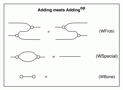
In our papers, Filippo, Fabio and I have been calling this system interacting Hopf algebras, or interacting Hopf monoids. The reason for the name is that the system of equations in the Adding, Copying, Adding meets Copying and the Antipode boxes is sometimes called a (commutative) Hopf monoid, as we discovered in Episode 18. The system of equations in the Addingop, Copyingop, Addingop meets Copyingop and Antipodeop boxes is a Hopf monoid again; the mirror image. And the remaining four boxes: Adding meets Addingop, Copying meets Copyingop, Cups and Caps, and Scalars tell the story of how these two Hopf monoids interact.

Altogether, there are quite a lot of equations, but there is a lot of symmetry going on. There’s quite a bit of redundancy as well: some combinations of equations imply the others. I will eventually write an episode that focusses on redundancy, but we are not going to be slaves to Occam’s razor. Let’s be honest with each other; conciseness and minimality was never a strong point of this blog.

The presence of symmetries is an important and interesting issue. Let’s account for two different ones. First, take any equation and invert the colours, swapping black and white; you get another fact, provable in the theory. This means that whatever theorem you prove, using diagrammatic reasoning, its “photographic negative” version is also true. We will take advantage of this symmetry quite a bit: it reduces your workload by half! Second, take any equation and look at in the mirror; it is also an equation of the system. So, whatever fact you prove with diagrammatic reasoning, its mirror image is also a theorem.

I want to leave you with one more observation. We have spent so much time talking about adding and copying… but looking at the equations, which ones tell us that the black structure means copying and the white adding? Well, we have just admitted that inverting colours is a symmetry of the system, so the answer must be… none of them. Copying and adding satisfy the same equations, and interact in the same ways. I still find this fact to be rather beautiful and mysterious.

There are several other, important properties satisfied by this set of equations, but I’ll save them for when they are needed. Most importantly: we know that the theory of Hopf monoids is isomorphic to the prop of integer matrices, so to give a diagram in that theory amounts to writing down a matrix of integers. So what linear algebraic notion does the theory of interacting Hopf monoids correspond to? I will leave you with this cliffhanger and save the explanation for the next episode, where we will also understand the algebra of fractions, diagrammatically.


I was in Cali, Colombia at the Javeriana university from the 25th of October to the 1st of November. I presented a tutorial on Graphical Linear Algebra at the ICTAC summer school, gave a talk at the Developments in Computational Models workshop, attended a whole bunch of inspirational talks, met up with some old friends and made some new ones. Everything was superbly organised and a lot of fun. Here’s a photo from my tutorial, where I seem to be demonstrating applications of graphical linear algebra to martial arts.

ictac

My favourite scientific talk was probably a mini tutorial by Jean-Raymond Abrial, also at the summer school, on doing maths with an “engineering” mindset. The idea is to capture the kind of process that goes on in a mathematician’s brain when writing a proof and formalise it (in a software tool!) as an instance of refinement, a software development concept popularised by Abrial and at the core of his B-method. Here’s a photo from that tutorial.

Abrial

Abrial demonstrated this by proving the Cantor-Schröder-Bernstein theorem in the Rodin tool. Here’s what I think, but first a disclaimer: I’m a theorem-prover/automatic-proof-assistant newbie. Also, I have to admit that I’m not a huge fan of the B-method in general: using sets and relations as building blocks is a bit too untyped and too low-level for my taste. Nevertheless, Abrial’s demonstration was intriguing. His discovery and distillation of the process of refinement in a mathematical context was quite compelling, and seemed to closely resemble “real mathematical thinking”, whatever that is.

At some point during the conference I was bragging to some of the attendees that I never suffer from jet-lag. Well, that was true up until now:I wrote about half of this episode after 1:30am, during a series of relatively sleepless nights spread over two weeks after returning from Colombia. I had jet-lag with a vengeance: I spent my days in a sleepy daze and got all my energy after midnight. Thankfully I’ve finally got back to normal over the last few days.

Continue reading with Episode 25 – Fractions, diagrammatically.

23. Frobenius Snakes and Spiders

separator

Graphical linear algebra is about the beautifully symmetric relationship between the operations of adding and copying numbers. The last episode was all about adding, the white structure of our diagrammatic language, using the new relational intuitions. Since copying, the black structure, is the yin to adding’s yang, in order to attain karmic balance we start this episode by shifting our focus to black diagrams. It turns out that the story is eerily similar: it’s the bizarro world all over again.

So, let’s take stock of what we know about copying. Here’s the generator that we already know quite well:

copyWith the relational interpretation, it represents the relation Num ⇸ Num×Num with elements

copyrelel

where x is any number. All this is saying, in the language of relations, is that the behaviour of the copying generator ensures that the three values on the dangling wires are all the same.

The relational interpretation of discard, copy’s sidekick

discard

is a relation of type Num ⇸ {}, but unlike zero from the last episode, it is not a singleton relation. Instead, it contains all elements of the form

( x, ★ )

where x is any number. This just means that discard, unlike backwards zero that “accepts” just 0, is not discriminating in the slightest.

From Episode 7, we know that copy and discard satisfy the commutative comonoid equations:

copying

And of course, these still make sense with the new, relational interpretation.


In the last episode we introduced the mirror image of the adding generator.This was backed by the relational interpretation; by thinking in terms of relations we could make sense of what it means to “add backwards”.

We can now do a similar thing with the copy and discard generators. We get a brand new generator, a backwards copy, or “copy-op”:

copyop

which, although not a function from left to right, is a relation of type Num×Num ⇸ Num. This relation is, as expected, the opposite of the one for ordinary copy:

copyoprel

The second new generator is the backwards discard

discardop

with relation { (★, x) | x ∈ Num }.

Not surprisingly, the mirror images of copy and discard satisfy the mirror versions of the equations for copy and discard.

copyingop


Now that we’ve seen both reverse adding and reverse copying, it’s natural to ask if anything interesting happens if these two structures meet. Back in Episode 8 we went through what happens when the ordinary versions of adding and copying meet.

So imagine you are standing in front of someone who is looking in the mirror. Do you get any more information from looking at the mirror than directly at the person? Typically not so much, the information is the same, but reversed. This is also the case for mirror add and mirror copy: they interact in the same ways, but backwards. Here’s a rundown of the equations; they are just the mirror image of the ones we discussed in Episode 8.

addingcopyingop


As in the case of adding, the interesting stuff happens when copying meets its mirror image. If you’ve just read the previous episode, the equation below will fill you with a sense of déjà-vu.

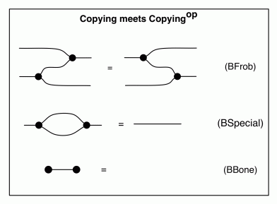
bfrob

Yes, it’s none other than a black version of the famous Frobenius equation.

In the last episode, to see that the white version of (BFrob) made sense, we had to do a few, admittedly simple, calculations. Here, the job is even easier: the copy generator carries the same value on all the wires; so tagging wires with the numbers that flow on them we see that the behaviour of the left hand side of (BFrob) ensures that all of the wires carry the same value.

froblvars

The story is similar for the right hand side of (BFrob).

frobrvars

In both the left and the right hand side of (BFrob), it’s thus quite simple to compute the underlying relation: it contains as its elements those pairs of elements that look like this

frobrel

where x is any number. The relations of the left and the right hand sides agree, so (BFrob) makes sense for copying.

So what other equations hold? Here’s another one that we’ve seen a few times by now: the special equation.

special

Again, just by looking at the thing, it’s pretty obvious that it works. On the left hand side of (BSpecial), the copy and it’s mirror image make sure that all the wires carry exactly the same value, meaning that the only behaviour exhibited is the one where the values on the dangling wires are the same. Which is the same behaviour as that of a single wire, the right hand side of (BSpecial).

Finally, we also have the bone, in black.

bbone

Summing up, we have identified three equations, just as we did in the last episode.

copyingcopyingop


Since we’ve now seen the Frobenius equation in two different contexts, it’s worthwhile to step back and see what interesting properties hold in Frobenius monoids, the algebraic structure that we mentioned briefly in the last episode. Stepping back and thinking more generally will help us get a better feeling for what’s going on under the hood. For the purposes of this discussion, we will switch to anonymous gray mode, remembering that the gray can be replaced either by white or black.

Here are the equations of Frobenius monoids again.

frobeniusmonoid

There are two interesting diagrams that can be built using the generators in any Frobenius monoid. First, we have a diagram with two dangling wires on the left and none on the right:

epsilon

and second, its mirror image, with two wires on the right and none on the left:

eta

Now, we can plug these two constructions into each other to form two different kind of “snakes”:

snakes

These two are involved in the snake lemma: both the snakes are actually equal to the identity wire. So, one intuitive way to think of  gadgets  and  is that they are a bent wire. When we compose such bent wires, we can stretch them back to get an ordinary straight wire.

snake

Here’s a proof of the second equality, which uses the Frobenius equation. The proof for the other equality is similar.

snakeproof

Because of the snake lemma, it turns out that any PROP with a Frobenius monoid structure is an instance of something called a compact closed category. Compact categories are all about bending things; we will say more about them in future episodes.


Maths is full of pretentiously sounding “fundamental theorems”, although perhaps this kind of language has become somewhat passé in recent decades. There’s the fundamental theorem of calculus, fundamental theorem of algebra, and a fundamental theorem of x for several other choices of x. The adjective fundamental is not really a precise classification; there is no definitive, widely accepted test of fundamentality. Rather, it’s more of a sociological endorsement that identifies a particular result because it holds some kind of spiritual, quintessential centrality for the field in question. A feeling that the point of view expressed by the theorem is a nice representation, a microcosm, of the subject as a whole.

Similarly, some people call the Euler identity e + 1 = 0 the “most beautiful equation” because it links, in one statement, some of the most important 19th century mathematical concepts: e, iπ, with timeless favourites 1 and 0. The 1 and the 0 may seem to be a bit contrived, and -1 seems to be getting a short shrift, why not e = -1? Not that I want to pick a fight with Euler.


It’s time for two particularly useful equations. In the spirit of pretentiousness and Platonic pompousness, we could call these the fundamental equations of graphical linear algebra, or the most beautiful equations, since they involve all of the generators that we have considered so far. But let’s not.

Here are the equations, which are mirror images of each other. Both feature the kind of “bent wires” that we were talking about before.

cc1

cc2

Let’s focus on  and calculate the relations. In the left hand side, we are composing the relation

addrel

with the singleton relation

zerorel

The operation of composition can be thought of as imposing a condition on the result of x+y.  Indeed, the composed relation consists of those elements

composed

where x+y=0. But to say that x+y=0 is to say that y=-x. In other words, the relation can be described as consisting of elements

final

where x is any number. But this is clearly the relation represented by the right hand side of , since the relational interpretation of the antipode is the relation with type Num ⇸ Num that consists of pairs (x,-x) for all numbers x.

 The justification for  is symmetric.


We have seen the snake lemma, it’s time for the spider theorem. It applies in special Frobenius monoids — those Frobenius monoids in which we also have the special equation. This, as we have seen, covers both the copying and the adding in graphical linear algebra. Here are the relevant equations.

specialfrobenius

In a very precise sense that we will eventually make clear, this theory, lets call it F, is dual to the theory we have been calling B, the theory of bimonoids. Remember that B consists of those equations that describes the interactions between adding and copying. Here’s a reminder of the equations, which by now we know quite well.

bimonoid

Back in Episode 16, when we were proving that a diagram in B is really the same thing as a matrix of natural numbers, we argued that diagrams in B can be factorised so that all the comonoid structure comes first, then the monoid structure: doing this made our diagrams look a lot like matrices. In F, the theory of special Frobenius monoids, the opposite thing is true: any diagram can be factorised so that all the monoid structure comes first, followed by all the comonoid stuff.

What this means is that any connected diagram from m to n is equal to the one in the picture below, where we use our usual syntactic sugar that collapses repeated multiplications and comultiplications:

spider1

This suggest an even better syntactic sugar for connected diagrams in special Frobenius monoids: a spider!

spider2

So—long story short—any diagram in F can be seen as a collection of jumbled up spiders: this result has become known as the spider theorem. Here’s an example with three spiders.

spidersex

Notice that if we have the bone equation around, we can get rid of the unfortunate legless spider. One more thing: when two spiders connect, they fuse into one spider. This is a really nice way of thinking about diagrams in F.

The spider theorem was proved by Steve Lack, in the paper Composing PROPs that we have already mentioned on more than one occasion. But later, it took on a life of its own, due to the usefulness of diagrammatic reasoning in quantum computing. The person probably most responsible for this is Bob Coecke; this paper with Eric Paquette is a good example of spiders in action.


It’s again been a pretty hectic few weeks for me.

Two weeks ago I was in Lyon for Fabio’s PhD defence. It’s now possible to download his thesis, which received high praise from the very impressive thesis committee. The thesis is currently the most thorough account of graphical linear algebra and its applications, so do take a look! After a well earned doctorate, Fabio has now moved to Nijmegen in the Netherlands to take up a postdoc.

Last week I was deep in paper writing mode, trying to meet the FoSSaCS deadline. If you remember Episode 2, this for me means pretty hard work. I get a bit too obsessive when writing, and the process takes up all of my time and energy: fortunately, the closer to the deadline, the more the adrenaline kicks in to keep you going. Deadlines are great at forcing you to get something done, but afterwards you end up feeling somewhat exhausted. So I tried writing for the blog this last weekend and it ended up feeling a bit too much like work, which is really not the point.

The paper itself, which has just been put up on the arXiv, is something that I’m really excited about. If you flick through it, I’m sure that you will recognise many of the equations! My coauthors are Brendan Fong, a brilliant PhD student of John Baez, whom we met in Episode 10, and Paolo Rapisarda, who is a control theorist in Southampton and an ex-PhD student of Jan Willems, whom we met in Episode 20. Academia is a small world. Anyway, it was a really fantastic collaboration; I very much enjoyed doing the research and I learned a lot from both Brendan and Paolo.

The paper is about the class of linear time-invariant dynamical systems, a foundational playground of control theory, where basic concepts that gave birth to the subject, such as controllability and observability, show up. In the paper, we give an equational characterisation—which means, for example, that questions about controllability can be reduced to looking at the shape of the diagrams that represent dynamical systems.

Next week I’m off to Cali, Colombia to talk about graphical linear algebra and its applications at the ICTAC conference. Then, hopefully, the noise will die down a little bit so that I can spend a bit more time on the blog.

Continue reading with Episode 24 – Bringing it all together.

22. The Frobenius Equation

After all the hype about relations in the last two episodes, it’s high time to use them to do something interesting. Let’s start by quickly reviewing the relational interpretation of our addition and zero generators. First, the addition:

add

Using our updated intuition, we are thinking of this as representing a relation of type Num × Num  ⇸  Num, defined as the set of all pairs

pairs

where x, y and z are any numbers that satisfy the condition x+y=z. So, for example, this relation contains the following three elements:

addexamples

The zero generator

zero

also has a relational interpretation. Its type is  {★} ⇸  Num. The reason for this is that Num0 is actually a singleton set—that is, a set containing precisely one element—and, since the name of this element does not matter, we may as well call it . The relational interpretation of the zero generator is the singleton relation

{(★, 0)}.        (‡)


The fact that Num0 is a singleton is related to a fact memorised by everyone in high school: we all know that k0 = 1 for any integer k. We will not spend a lot of time getting very deep into this now; let me just say that it’s one of the things that category theory can explain really well, maybe even better than people on Quora. I will just outline the basic idea—and if the following is too technical, don’t worry, it’s not important for our story.

The cartesian product of sets is an example of a general phenomenon called a limit. Binary, tertiary, and n-ary cartesian products (sets of pairs, triples, n-tuples, and so forth) are particularly simple instances: they are limits indexed by very simple categories.

For example, binary cartesian products are limits indexed by a category with two objects and only identity arrows. Such very simple categories, where there are no non-identity arrows, are sometimes called discrete.

Then, n-ary cartesian products are limits indexed by a discrete category with n objects. So what is a zero-ary cartesian product? A limit for the discrete category with no objects (i.e. the empty category) has its own name: it’s called a terminal object. And, in the category of sets, any singleton does the job of being terminal.


One of the things that you can do with relations that you can’t, in general, do with functions is turn them around. The result is sometimes called the opposite relation. We can use this idea to make sense of the following new generator, which looks like the mirror image of addition:

addrev

We will be thinking of this strange new beast as representing “addition backwards”. Although that does not make much sense as a function from left to right, it makes perfect sense as a relation; it is the one that consists of pairs

pairsrev

where x, y and z are any numbers that satisfy x+y = z. Of course, this is just (†), but backwards.

We can also reflect the zero generator to get a new generator that looks like this:zerorevThe relation this generator represents is, not surprisingly,

{(0, ★)}

which is just (‡) backwards.

As we do more graphical linear algebra, you will see that these mirror versions of addition and zero are extremely useful to have around!


Back when we were talking about ordinary addition, we identified some equations that concern the addition and zero generators. These were (Comm), (Unit) and (Assoc), and here they are again:

adding

Since the backwards addition is still addition, it satisfies the same equations, but backwards.

addingop

It’s useful to notice that these end up looking a lot like the equations for copying; here they are again, as a reminder:

copying

In fact, the equations for adding backwards and copying are exactly the same, apart from the colouring of the nodes. The colours make sure that we don’t confuse backwards addition and copying, since our intuition is that they stand for different relations. Also, again in order to avoid confusion, we tag all the new equation names for with op, for opposite. We will come back to copying, viewed relationally, in the next episode.

The equations for backward adding are not controversial. In fact, they are rather boring, and we have not really discovered anything new about addition so far. The interesting, new stuff comes when we think about what happens when addition sees itself in the mirror.


So what happens when we connect the adding generator to its mirror image? Let’s focus on the most interesting examples first, and concentrate on the relation represented by the following diagram:

frobleft

We could translate everything back to first principles and compute the composition as in Rel, but just by looking at the diagram it’s clear that there are three variables involved; the numbers on the three wires that connect as arguments to the two additions. Let’s call these x, y and z and label the wires accordingly:

frobleftann

So, the relation consists of pairs

frobleftrel

for all choices of x, y and z. For example, taking x=1, y=-1 and z=3, we see that

frobleftex

is in. Another example, taking x=3, y=2, z = -5 gives us

frobleftex2

Looking at these examples, it seems that there may be another way of describing these pairs: those in which if we add the components, we get equal sums. Indeed, in the examples above we have 1+2 = 0 +3 = 3 and 3+-3 = 5 + -5 = 0.

So let’s see if is actually the same relation as ② below, which consists of all pairs

frobmidrel

where p+q = r+s. Incidentally, ② is the relation represented by:

frobmid

Just by looking at  and , clearly every  is an instance of , since summing up either of the two components of  gives x+y+z. Then to show that  and  are the same relation, it’s enough to to show that every instance of  is an instance of .

So lets take a closer look at . Since p+q = r+s, we can express each variable in terms of the other three, so in particular q=(r-p)+s and r=p+(q-s). This is almost in the form required by , we just need to show that r-p = q-s and indeed:

r-p = p+(q-s)-p = q-s.

That finishes the job:  and  denote the same relation. These arguments give us the justification for introducing the following intriguing equation.

frob1

In fact, the argument above can be recycled to show that also

frob2

since the calculations involved are clearly symmetric.

A nice way of memorising  is that it says “Z = X”: the diagram on the left looks a bit like the letter Z and the one on the right looks like an X. Then, the mnemonic for  says, for similar reasons, that X = S. Together, we have Z = X = S, and so in particular Z = S.

frob

These three equations are quite famous; they are called the Frobenius equations. It’s a little bit redundant to keep all three, because it turns out that all three of (Frob),   and  are equally powerful: any one one of them lets you prove the other two, using diagrammatic reasoning. So, out of the three, we will just keep (Frob) because it is the most symmetrically pleasing.

For example, below there is the proof of , assuming that we have (Frob). I’ll leave the other five implications for you as nice exercises!

frobproof

By the way, structures satisfying these equations, repeated below in an anonymous, gray mode, are often referred to as (commutative) Frobenius monoids.

frobmonoid


Ferdinand Georg Frobenius was a German mathematician, active in the late 19th and early 20th century. He was very good, but he also happened to have an extremely cool last name. These two facts combined mean that a surprisingly large number of mathematical notions are called after him. He also had a pretty inspirational beard, as verified by the following photo.

Frobenius

The Frobenius equation (Frob) is probably most famous for the role it plays in the impressively named and difficult-sounding field of 2-dimensional topological quantum field theories (2D TQFT – even the acronym is scary!). There’s a very nice book on the subject by Joachim Kock called  Frobenius algebras and 2D topological quantum field theories. You can’t say that the title is misleading. And 2D TQFT, despite the name, is actually not that difficult to get your head around. A bit like the Sierpinski space.

Frobenius didn’t actually discover the Frobenius equation. As is often the case, there is a bit of controversy about who exactly thought of it first. Mathematicians can get quite uppity about this sort of thing. Some mathematics message boards descend into mini flame wars as people argue about what exactly was written in the corner of some blackboard at an obscure conference somewhere off the coast of Britain in the mid 1960s. I guess that professional mathematicians are amongst the very few people who actually remember any details of that particular decade.

My feeling is that—as is not uncommon with good maths—it’s likely that number of people thought of it at around the same time. The Frobenius equation was in the air. And it’s going to be a favourite of ours on this blog.

Having said all that, one of the earliest people to realise the importance of the Frobenius equation was Bob Walters, who I’ve talked about in Episode 12. If you’re interested in some of the history, you can take a look at a blog entry of his here where he wrote about some of its history. Note that Bob talks about the equation X=S, our equation . But as we’ve discussed before, it doesn’t matter which one of (Frob) or  you consider.


There are two more equations that show interesting ways in which addition interacts with itself in the mirror. We have already seen the first one in the last episode, where it featured as one of the equations of the special bimonoid, the structure isomorphic to the PROP of relations. It is none other than the “special” equation. Unfortunately the name “special”—terrible as it is—seems to have caught on, so we are stuck with it. Here it is:

specialLet’s convince ourselves why it makes sense in our context of addition interacting with its mirror image. Doing the simple calculation, the left diagram represents the relation

{ (x, y) | there exist numbers u, v such that u+v = x and u+v = y }.

Now, given any element (x, y) in this relation, it’s easy to see that x = y, since they are both equal to u+v for some u and v. Also, for any number z, (z, z) is in the relation because we can take, for example, u = z and v = 0. These two arguments combine to mean that the relation is actually the identity relation

{ (x, x) | x is a number }

which is, of course, the relational meaning of the identity wire. So, long story short, (Special) is compatible with our intuitions.

The second equation, (WBone), is pretty self evident: it’s the white version of the bone law from Episode 8. Both of the diagrams in (WBone) represent the relation that contains the single element (★,★).

wbone

The table below summarises the equations that we have discussed in this episode, which capture the various ways in which addition interacts with its backwards twin.

addingaddingop


Unfortunately, the rate of articles has slowed down somewhat recently. This is mainly due to the time of the year: it’s the start of semester, so teaching, supervision and related activities are taking up a lot of my time.  Also, coincidently, this is the time of year when there are a few paper deadlines. And on top of all that I have a few pretty exciting research leads to chase. I’m sure that some of these will make it on the blog eventually.

I hope that the pace will pick up again in October. If you’ve stuck with the series so far, let me just say that we are getting very close to the really interesting stuff!

Continue reading with Episode 23 – Frobenius Snakes and Spiders.

21. Functions and Relations, diagrammatically

There is a cute graphical/algebraic way of understanding functions and relations between finite sets, and it deserves to be more widely known. The (formal) diagrams involved closely resemble the (informal) pictures that lecturers often draw when first explaining these concepts to undergraduates.

Although somewhat tangential to the main spine of the story of graphical linear algebra, the diagrammatic treatments of functions and relations give us two additional, simple examples where well-known mathematical structures are characterised as free PROPs. We have already seen two examples: the isomorphisms between Mat and B (Episodes 15 and 16) and between MatZ and H (Episode 19). We will see several more in future episodes.

Now is a good time for a discussion about functions and relations: as we discussed in the last episode, relations play a very important role in graphical linear algebra; this episode thus also serves as a little primer/reminder.


First, let’s fix some notation. A bold number n represents a finite set that contains the elements 0, … , n-1. So for example

1 = { 0 },  2 = { 0, 1 },  = { 0, 1, 2 }

and so on. 0 is the empty set, that is, it has no elements.

A function f from m to n, often written f: m → n, is a kind of “rule”; we can evaluate it by giving it an element k in m (i.e. 0 ≤ k < m). The result is denoted f(k) and it is an element in n  (i.e. 0 ≤ f(k) < n).

The definition does not specify how f works, and a function is considered to be equal to another precisely when the two have the same domain and codomain, and act the same way on all possible inputs. This is sometimes called the extensionality property of functions: in more mathematical jargon, if f and g have the same type, we have that:

 ∀x. f(x) = g(x)  implies  f = g           (extensionality)

So the only interesting information about a function is (1) its type and (2) where it takes each of its arguments.


I remember that when I first encountered the notion of function, I found it a bit weird. Shouldn’t there at least be some kind of formula or algorithm that calculates it? The functions that I remembered from high school always had a rule, and usually a simple one, say f(x) = x2.

I also remember finding the extensionality property strange at first. I can write two very different computer programs to calculate, say the factorial of a natural number. Extensionality says that they are considered to be the same thing when thought of as functions. So, if you like to think in terms of algorithms, it can be useful to think of a function as a kind of idealised specification, which may have zero or more implementations.


There are finitely many functions from any finite set to another. To get the total number of functions from m to n, the crucial insight is that we only care about where the elements from the domain go. We have n choices where to send 0, n choices where to send 1, etc. Since each choice is independent, the total is just n multiplied by itself m times, i.e. nm.

For example, here are pictures of the four functions from 2 to 2.
22functions

Let Fun denote the PROP where the arrows from m to n are functions from m to n. Composition in Fun is composition of functions: if f: m1 → m2 and g: m2 → m3 then their composition, often written g ○ f or f ; g is a function m1 → m3. We just apply one rule after the other:

(g ○ f) (k)  :=  g(f(k))

Pictorially, this means plugging in the output of the first function as the input of the second. So for example, composing the “twist” function with itself is the function

composition

which is the identity, by extensionality, since each argument ends up being taken to itself.

The monoidal product in Fun is similarly simple: it is “stacking one function on top of the other”. Pictorially, this is very simple to visualise, e.g.

funproduct

We can write a somewhat less enlightening formula for this. If f1: m1→n1 and f2: m2→n2 then

funproduct
The permutations of Fun are the obvious things–they are simply traditional permutations, viewed as functions. And it is not difficult to show that all the properties required of PROPs hold.


So what is the theory that characterises Fun? It turns out that we have met it already on this blog.

monoid

Let’s call the PROP that arises from the equations above M. Then M and Fun are isomorphic as PROPs. By the way, in this episode we colour all diagram nodes gray: this is so that we don’t get our intuitions confused, since our convention is that the white structure is “adding” while the black structure is “copying”.

The proof that M is isomorphic to Fun is not very difficult, but we will skip it for now. We will probably come back to it when discussing distributive laws, because they also rear up here. For now, to convince you that this has a chance of being true, I’ve drawn the diagrams that represent each of the functions from 2 to 2 that we enumerated previously.

fundiags

See what I meant about the diagrams looking very much like the pictures one draws of functions?

The isomorphism between M and Fun means that to give a function from m to n is the same thing as to give a diagram in M. And two diagrams are equal via diagrammatic reasoning exactly when they define the same function.


I took discrete maths course as a first year undergrad. That’s where I first encountered functions in the abstract, set theoretical sense.

Taking discrete maths was a fun experience, and challenging in some ways; even though the computations were not very complicated, it was my first exposure to abstract mathematics. We went through the basics of naive set theory, including the notions of cardinality, functions and relations, then went on to matrices, vector spaces, simple combinatorics, etc. I guess that the recipe is similar in most maths/CS degrees around the world.

Five years ago I found myself having to teach them in a Southampton variant of a discrete maths course. And I found out that teaching discrete maths, which I expected to be a breeze, is actually quite challenging.

In fact, the whole idea of abstract, untyped sets and basic operations on them can be quite strange for students straight out of high school. Once they get the basics though, functions are a breeze. But when we get to relations… there’s always trouble. And no matter how much time I spend on them, it seems that for some people it’s difficult to grasp; even when I keep repeating “remember, a relation is simply a subset of the cartesian product”.

I think that it’s got something to do with psychology: people already have a feel for functions, even before they know the formal definition. Rules are something familiar, it’s that inputs and outputs idea again. The world of relations, in comparison, seems strange and much less intuitive—even if the definitions are extremely simple.


If X and Y are sets, then a relation R from X to Y, written R: X ⇸ Y, is a subset of the cartesian product X×Y. What this means is that R is a collection of pairs of the form (x, y) where x is an element in X and y is an element in Y.

Just as with functions, it’s pretty easy to count the total number of relations between finite sets. For example, to figure out the number of relations from m to n, first we observe that the total number of pairs (x,y) where x is in m and y is in n is simply mn, since there are m choices for x and n choices for y. Second, a relation is a subset of the cartesian product, and a finite set of cardinality k has 2k subsets. It follows that there are 2mn such relations.

Let’s draw the relations from 2 to 2, there should be 24 = 16 of them. In the pictorial representation, a line connects x to y precisely when (x,y) is in the represented relation.

relationsann

There is one interesting thing to notice: if you look at the pictures of functions → 2, we can find similar pictures amongst the relations:  (h), (i), (j) and (k). This is because every function from m to n can be thought of as a relation. This relation is sometimes called the graph of the function, and it’s defined to be the subset { ( k, f(k) ) |  0 ≤ k < m }. It’s therefore quite natural to think of functions as special kinds of relations.

The PROP where arrows from m to n are relations from m to n is called Rel. Composition in Rel is, as expected, composition of relations. If you haven’t come across this before, it’s very simple. If R: m1 ⇸ m2 and S: m2 ⇸ m3 then R ; S is the relation m1 ⇸ m3 defined:

R ; S = { (x,z) | there exists y such that (x,y) ∈ R and (y,z) ∈ S } 

Again, pictorially, this is pretty simple to explain: we put the two relations we are composing side by side, and include a connection from the starting point to the end point if there is a path that takes us there. We don’t care about the precise number of paths, as long as it’s greater than 0. Here are some examples:

relcomprelcomp2

relcomp3

As we observed before, every function gives rise to a relation, and it’s not difficult to see that relational composition is compatible with composition of functions: if I compose two functions and look at the resulting relation then it is the same one as if I composed the two functions as relations.

The monoidal product in Rel is also similar to the one in Fun: again, we stack relations on top of each other. For example:

relproduct

The permutations are the graphs of permutations. Again, it’s not difficult to verify that Rel satisfies all the conditions required of PROPs.

The fact that composition and monoidal product are compatible in Fun and Rel can be captured succinctly by the observation that there is a faithful homomorphism Fun → Rel. Obviously this homomorphism is not full, because, in general, not every relation from m to n is the graph of a function.


As was the case with functions, we have also seen almost all we need to understand how to characterise relations diagrammatically. The theory that does the job is the following.

special

We have seen most of these equations before. Taking (S) away, it is just the theory B, and we went though all of its equations in detail in Episode 8. We know that B is isomorphic to the PROP Mat of natural number matrices.

The equation (S) is sometimes called the “special” equation. It’s not a great name, but it seems to have stuck so we will use it. If we think in terms of natural number matrices, (S) seems to be saying that

2 = 1

which may look… a bit weird. But, thinking about the graphical interpretation it makes sense. We saw in Episode 9 that the diagrammatic way of understanding natural number matrices has to do with counting paths. Similarly, when composing relations we also have to keep track of paths, it’s just that we are only interested in the Yes or No question “Is there a path?”, and we don’t care about the number. This is one interpretation of (S): it ensures that having 100 paths is the same as having 1 path (but different to no paths).

Again, we won’t prove that the PROP generated by the theory of special bimonoids is isomorphic to Rel. Let’s save that for later. For now, here is a picture of how some of the pictures of relations from before look as diagrams in the theory.

relpics


I wrote a part of this episode during my holidays on a train from Yerevan, the capital of Armenia, to Tbilisi, the capital of Georgia. The train trip was quite an experience.

It was an old Soviet relic from I would guess the 60s or the 70s. The weather was very warm, in the high 30s, but fortunately the train was equipped with air conditioning. Unfortunately, it was controlled by a matronly, but friendly, Russian lady who was in charge of the carriage. If she judged that the sun was not shining hard enough, she simply turned the aircon off and walked along the corridor, opening windows. Once the train heated up (way) past the point of comfort, the ritual was reversed.

train

The toilet wasn’t too pleasant and there was no running water. But; surprise! Fast, free public wifi.

One last thing. We are looking for PhD students!

Continue reading with Episode 22 — The Frobenius Equation.

20. Causality, Feedback and Relations

This is an important episode in the story of graphical linear algebra. We return to our intuitions, the ones we started with all the way back in Episode 3. It’s high time we replace them with something much more useful.


In our diagrams so far, we have been saying that numbers travel on the wires from left to right. By the way, all along, we have been rather vague about what these numbers are exactly — and as we expanded our set of generators and their associated equations, we have been getting more specific. So far, we know at least that we have a zero (which is part of the addition structure) and negatives (the antipode).

Let’s call the type of these numbers, whatever they are, Num. Then the addition generator defines a function of type

Num × Num  →  Num

add

since there are two arguments x and y (the numbers that arrive on the input wires on the left) and one result x+y (the number that exists on the the output wire on the right). Similarly, we could write down the types for all of the other generators. And in our algebra of diagrams, the composition operation always connects outputs to inputs.

Every diagram thus defines a function that takes a certain number (possibly zero) of inputs to a number (possibly zero) of outputs. In other words, every diagram that we drew conforms to the following idealised—and pretty cliché—idea of a computational system. The picture below could appear in a million papers and talks in computer science and related fields.

system

We could even go so far as to say that the inputs we provide are causing the outputs. Let’s not go down that road; it causes a lot of problems. Let me explain why.

(A warning: the rest of this episode is about 90% rant; if you just want the content, feel free to skip to the last section.)


Causality is an enchanting, seductive idea. Imagine: we interact with the world by giving it inputs, and the world responds by returning nice, easily predictable outputs. Life would just be so easy and pleasant if everything around us behaved as functions in the mathematical sense: for every input x there would be an output f(x). And, the cherry on top, imagine if f had a closed form. A nice little theory of everything.

Unfortunately, reality is somewhat more brutal. In 1912, the year the Titanic sunk, Bertrand Russell published a very nice philosophical paper entitled On the notion of cause. It is full of delightful quotes, and here is one of my favourites:

The law of causality, I believe, like much that passes muster among philosophers, is a relic of a bygone age, surviving like the monarchy, only because it is erroneously supposed to do no harm.

Clearly, Russell was a republican. But his paper is mainly a scathing attack on the facile idea of causality: viewing the various components of the physical world as cause-and-effect systems.

Of course, it is extremely useful to engineer systems that behave in a cause-and-effect manner: our carefully constructed civilisation relies on it. If you buy a car, you would not be very happy if nothing happened as you pressed the accelerator pedal. Similarly, a lamp should do something when you flick the switch. Clearly we are causing the car to go and the light to go on by interacting with those systems appropriately.

The problem arises when we try to use our fuzzy “common-sense” human intuitions of causality to understand the physical, non-manufactured world around us, or even the sub-components of engineered systems. Causal preconceptions affect the way we approach reality: to get the outputs we want, all we need to do is find the right inputs. When a person with this world view sees something happening, they ask why, what caused it? This question may seem quite reasonable at first.

Quoting Feynman:

Aunt Minnie is in a hospital. Why?

Because she went out, she slipped on the ice and broke her hip. That satisfies people.

If you haven’t seen it, go ahead and watch the video, it’s very entertaining. Feynman is addressing the difficulty of answering a question like “Why do magnets repel each other?”One of the messages of the video is that it is difficult to apply “common-sense” to understand the physical world. In “common-sense” the questions “why?” and “what caused it?” are closely linked. And the idea of something causing something else, away from our carefully engineered human civilisation, becomes more flimsy the more one thinks about it.

But maybe this world view is harmless, like the monarchy? They (the monarchy) do bring in loads of tourists, after all. So maybe causal thinking gets us to ask the right questions, e.g. Newton and the Apple incident. What caused the apple to fall?

Not quite. Causality encourages sloppy thinking that is far from harmless: it is killing people, while costing billions in the process. If this sounds like an outrageous hyperbole, a cautionary tale is recounted in Jonah Lehrer’s article Trials and errors: Why science is failing us. Check it out, despite the clickbait title it’s worth a read. Full disclosure: Lehrer is an interesting guy. He seems to have been transported to life from a stock character in some Shakespearean play: first a stratospheric rise from science blogger to best-selling author with a cushy staff writer gig for the New Yorker. Then an equally steep fall from grace—apparently he faked some Bob Dylan quotes for one of his books—so spectacular that it merited two chapters in Jon Ronson’s So you’ve been publicly shamed.  But let’s not throw out the baby with the bath water.

Lehrer writes that in the early 2000s, Pfizer, the multi-billion dollar pharmaceutical company, pumped a lot of money into the development of a drug called torcetrapib, which tweaked the cholesterol pathway—one of the most studied and seemingly well-understood systems in the human body—to increase the concentration of HDL (“good cholesterol”) at the expense of LDL (“bad cholesterol”). Here’s a diagram.

cholesterol

It actually did exactly that; increased HDL and decreased LDL. But there seems to be a deeper problem concerning the diagram above: the simplification involved in considering some chemical as a “good input” and another as a “bad input”. Long story short, quoting Lehrer:

Although the compound was supposed to prevent heart disease, it was actually triggering higher rates of chest pain and heart failure and a 60 per cent increase in overall mortality. The drug appeared to be killing people. That week, Pfizer’s value plummeted by $21 billion (£14 billion)

It’s pleasant and probably quite lucrative—research grant wise— to call HDL “good” and LDL “bad”.  It seems likely, however, that they are not inputs in any useful sense; they are components of a complex system, the cholesterol pathway, which is part of a larger, more complex system, the human body.

Causal thinking and complex physical systems don’t mix very well. Still, the causality meme is as strong as ever, more than 100 years after Russell’s paper. A wonder drug (input) that cures cancer (output) is just around the corner. But you need to donate now.

So what is it about complex systems that makes them so difficult for humans to understand? Why is it that HDL or LDL might not be inputs in any meaningful sense? And what does all of this have to do with graphical linear algebra?


One of the most famous, the most studied, and yet the most mysterious features of complex systems is feedback: the somewhat circular idea that an output of a system can be plugged back in as an input. So, suppose that we have a nice, easy causal system with two inputs and three ouputs, as follows.

system2

Now, what happens if I plug the first output in as the first input? I get the following system which now seems to have only one input and two outputs.

feedback

The idea of recursion, which we have seen in many of our syntactic sugars, is related and similarly circular: we used the sugar within its definition. It maybe made your head spin at first, but as long as one is careful, recursion is extremely useful. Similarly with feedback; and nature has figured this out. Many physical systems have feedback loops of some kind. Cholesterol—surprise!—is regulated by a feedback process.

Look again at the diagram above: three out of the four wires seem to be straightforward; they are either inputs or outputs. But what is the status of the feedback wire: is it an input or an output? What about the data that passes along it, numbers, bits, cholesterol, force, charge, whatever? Is that data an input or an output? This is one place where the input/output causal analysis begins to fall apart.


So how did we create our causal civilisation, with cars, trains and lamps, from a non causal physical world? Of course, this is where engineering comes in, and at the science end of engineering it is the topic of an entire field of study, control theory.

Control theory has undergone a little anti-causality revolution in the last thirty years or so, with the emergence of a subfield called the the behavioural approach. Its visionary creator, Jan C. Willems, wrote a bunch of fantastic papers on the subject. A good one to start with is The Behavioral Approach to Open and Interconnected Systems. Willems is immensely quotable, and here’s one quote from that paper:

It is remarkable that the idea of viewing a system in terms of inputs and outputs, in terms of cause and effect, kept its central place in systems and control theory throughout the 20th century. Input/output thinking is not an appropriate starting point in a field that has modeling of physical systems as one of its main concerns.

I would go so far as to claim that graphical linear algebra is the behavioural approach applied to linear algebra. We will discuss what I mean by this, as well as some of the contributions of Willems and the behavioural approach in future posts on the blog. The connections with control theory will become especially apparent when we will use graphical linear algebra to explain the behaviour of signal flow graphs; a formalism used in the study of time-invariant linear dynamical systems.

I just want to address one last point before we get to the content. Why does a guy whose job it is to understand input/output systems rail against inputs, outputs and causality? Isn’t this a little bit like a car manufacturer advertising the merits of bicycles?

Not quite: and the hint is in the quote. What Willems doesn’t like is taking inputs and outputs as the starting point. In more mathematical slang: Willems doesn’t want inputs and outputs as definitions, as assumptions that we make about physical systems, because they are a dangerous fiction—the real world simply doesn’t pander to our sociological, evolutionary hang-ups. Inputs and outputs are more like theorems, they exist because we carefully craft systems so that some variables behave as we would expect inputs or outputs to behave.


Let’s go back to our intuitions, with a view to getting rid of our functional hang-ups.

It’s actually pretty simple: instead of thinking of our addition generator as a function of type  Num × Num  →  Num we will view it as a relation of type Num × Num  ⇸  Num.

add

If you have not seen relations before, I will briefly explain the basics in the next episode. And we will start to see what the change in perspective in allows us to do. For now, just a brief taste.

By moving from functions to relations we are no longer thinking of the gadget above as taking two inputs to an output; we are thinking of it as determining a kind of contract: the only behaviours allowed by the addition generator are situations where numbers x and y appear on the left and x + y appears on the right.

This means that we loosen the causal associations: we can no longer simply say that the two numbers on the left are inputs and the number on the right is an output.

add1

In fact, for the addition generator, if I know the values on any two wires I can figure out the value on the third. For example, if the value on the first left wire is 2 and the value on the right wire is 1 then I can figure out from the contract that the value on the second left wire is -1, since 2 + -1=1. So we can quite reasonably also consider the first left wire and the right wire as inputs and the second left wire as an output.

add2

But instead of tying ourselves up in knots, it is just better to just stop using the words inputs and outputs for now. We will come back to them only when they become useful.


I gave a tutorial on graphical linear algebra at QPL ’15 two weeks ago. I just about managed to finish the slides on time! If you want a preview of what’s coming up on the blog you can take a look here. The videos of my talks will be released on the Oxford Quantum Group youtube channel; the ones that are there currently cut off after 1 hour, but this will be fixed soon.

I’m also going holidays starting next week, so the next episode will likely arrive sometime in early September.

Continue reading with Episode 21 – Functions and relations, diagrammatically

19. Integer Matrices

In the last episode we introduced the fifth and final principal actor of graphical linear algebra, the antipode. This episode’s main task is showing that diagrams built up of the five generators constitute a diagrammatic language for integer matrices and their algebra. We will also discuss a cute example involving the complex numbers.

The cheat sheet for the diagrammatic system H  that includes the antipode is repeated below for easy reference.

cheat

We have already showed that H allows us to extend the syntactic sugar for natural numbers to a sugar for all the integers. We have also verified that the integer sugar obeys the usual algebraic laws of integer arithmetic. In particular, we proved that

minusonesquared

using the equations of H and diagrammatic reasoning: this is just -1 ⋅ -1 = 1, expressed with diagrams.


Let’s start with an example. The diagram below has two dangling wires on both sides.
iAs such, it ought to denote some 2×2 matrix, and to get the entry in the ith row and jth column we need to look at the paths from the jth dangling point on the left to the ith dangling point on the right.

Before the antipode entered the frame, it sufficed to count the number of paths; the current situation is a little bit more complicated because there are positive paths—those on which the antipode appears an even number of times—and negative paths, those with an odd number. To get the relevant integer entry, we need to take away the negative paths from the positive paths. So, in the very simple example above, we have exactly one positive path from the first point on the left to the second point on the right, and one negative path from the second point on the left to the first on the right. The corresponding matrix is therefore:

imat

Actually, I didn’t choose this matrix at random: it allows us to consider the complex integers (sometimes called the Gaussian integers) and their algebra in a graphical way. We will come back to this after tackling the main topic for today.


We want to prove that H is isomorphic to the PROP MatZ of matrices with integer entries. The letter Z is often used to mean the integers, from the German word Zahl meaning number; this notation was apparently first used by Bourbaki.

MatZ is similar to the PROP Mat that we discussed in Episodes 12 and 13: the arrows from m to n are n×m matrices, and just like before composition is matrix multiplication. The monoidal product is again direct sum of matrices.

The proof H ≅ Mat(the symbol  is notation for isomorphic to) is similar, and not much more difficult than the proof, outlined in Episodes 15 and 16, of ≅ MatLet’s go through the details.

First we define a homomorphism of PROPs from H to MatZ. Let’s call it φ, the Greek letter phi. Since both H and MatZ are PROPs, and H is a free PROP built from generators and equations, it is enough to say where φ sends all the generators, and then check that the equations of H hold in MatZ.

It turns out that φ works the same way as θ for all of the old generators. The new part is saying where the antipode goes, and not surprisingly, it is taken to the 1×1 matrix (-1). Like so:

phi

For φ to be well-defined, we need to check that all the equations of  H also hold in MatZ. Fortunately, most of that work was already done for θ, we only really need to check the new equations that involve the antipode. Let’s check the most interesting of these, (A1); we need to calculate whether the following is true:

phia1

This amounts to checking if

phia1t

and it does, indeed, work. The other equations, (A2) through to (A5) are similarly easy computations and we will skip them; but feel free to check!


So we have a homomorphism φ: H → MatZ. To show that it is an isomorphism, we will show that it is full and faithful. Fullness—the fact that every matrix has a diagram that maps to it via φ—is the the easy part.

First, we need to check that the sugar that we defined in the last episode works with φ as expected, which is confirmed by the following simple calculation:

negsugarv

Any matrix with integers as entries can now be constructed following the procedure described in Episode 15. We will skip the details, as it is all pretty straightforward! The upshot of the construction is that we can extend the sugar for natural number matrices to a sugar for integer matrices: given an m×n integer matrix U we obtain a sugar

matrixsugar

such that

fullness

This establishes that φ is full.


So what about faithfulness, the property that says that whenever two diagrams map to the same matrix then they must already be equal as diagrams?

The trick is to get our diagrams into the form where the

copying comes first, then the antipodes, then the adding  (★)

One way of doing this is to use the theory of distributive laws. Eventually we will go through all of this properly, but for now I will just give you a high-level executive overview. The main insight is that we have three different distributive laws, the first involving the adding and the copying (B1)-(B4), the second the antipode and copying (A2)-(A3), and the third the antipode and adding (A4)-(A5).

The three distributive laws, are compatible with each other in a sense identified by Eugenia Cheng in her paper Iterated distributive laws. The fact that the distributive laws play together well in this way gives us the factorisation (★) that we want. We will discuss Cheng’s results in more detail in a later episode. Incidentally, she has recently written a book about category theory and recipes; I wonder if she knows about Crema di Mascarpone!


We could also try a rewriting argument, taking for granted that the rewriting system described in Episode 16 terminates.  Adding the following rules

rew

it seems that the expanded system ought to terminate also, although I have not yet got around to proving it. These termination proofs are always really messy for a rewriting amateur like me; I would love to hear from an expert about how to do these kinds of proofs in a nice way.


Once we know that every diagram can be put in the form (★), the proof of faithfulness is fairly straightforward. We start with those diagrams that have one dangling wire on each side. Every such diagram in the form  (★)  is either the sugar for 0 (a single discard followed by a single zero) or it can be rearranged into the form:

1-1

for some natural number k of wires with one antipode and some natural number l of wires with no antipode. This is because we can always get rid of redundant discards and zeros with (Counit) and (Unit), cancel out multiple antipodes in series using (†), then rearrange, and eat up any annoying permutations with the iterated copy and add sugars.

Once our diagram is in this form we can desugar and repeatedly use (A1), each time destroying one pair of antipode wire and no-antipode wire. Either we end up with no antipodes left, in which case the diagram is equal to a non-negative sugar, or we end up with some number of antipode wires. In the latter case, we can use (A2) to pull out the antipode to the left, obtaining the sugar for a negative integer. We have thus shown that faithfulness holds for the (1,1) case, since every such diagram is equal to some integer sugar.

The general case, where diagrams can have any number of wires on the left and right, comes down to transforming the diagram in matrix form, as explained in Episode 16. This step completes the proof that φ is faithful, and since we already know it is full, it is an isomorphism.


So far we have been identifying “numbers” with diagrams of a particular kind; those with one dangling wire on each end. In B this gave us the natural numbers, and in H it gives us the integers. But, as argued in Episode 17, there’s nothing particularly special about (1, 1) diagrams; well, maybe apart from the fact that both in B and H composition for (1,1) diagrams turns out to be commutative. Our obsession with the (1, 1) case is due to history—the traditional way of doing matrix algebra means the concept of ‘number” comes first, then the concept of “matrix”.

The complex numbers are a nice example where it makes sense to consider “numbers” as something different than (1,1) diagrams  A complex number can be written as an expression r + si where rs are numbers and i is a formal entity that behaves like a number, but with the mysterious property i= -1. The numbers and s are sometimes called, respectively, the real component and imaginary components. What is important for us is that to describe a complex number, it suffices to keep track of two ordinary numbers.  Our intuition is that wires carry numbers, so it makes sense to carry a complex number with two wires, the first for the real piece, the second for the imaginary piece.

complexintuition

Now if we multiply a complex number r + si by i, we get (r + si)i = ri + sii = -s + ri. So what was the real component becomes the imaginary component, and the negative of what was the imaginary component becomes the real component. We have a diagram for that, and we have already seen it in this episode:

iint

It thus makes sense to call this diagram i:

idef

Now if we multiply r + si by an integer u, we get (r+si)u=ru + sui. So both the components are multiplied by u. We also have a diagram for that:

scalarsugar2

where on the right hand side we used the sugar for integers from the last episode.

For the rest of this section, to stop the proliferation of the digit 2 that clutters the diagrams, we will just draw the 2 wire using a thicker line, like so:

thick

Now we can do some calculations. First if we compose the diagram for i with itself we get:

isquared

We can also show that i commutes with integers:
icommutes

Following the general pattern of this blog,  we can ask what kinds of diagrams one can construct using the following gadgets.
componentsUsing our standard box of tricks for reasoning about diagrams, it is not difficult to show that the diagrams with one thick wire on each side will, in general, be of the form:

gaussint

Composing two such entities gives us

gaussianmult

which is of course what you’d get if you multiplied out two complex integers (those complex numbers u+vi where u and v are integers). In general, the diagrams that can be constructed from bricks (‡) are matrices with complex integer entries.

So what exactly is going on here? Let’s take a look under the hood.

hood

The result is in matrix form, and corresponds to the 2×2 matrix:

mat

and this is known as one way of representing complex numbers using matrices.

There is one more interesting thing to say here. Let’s take a look at the bizarro of i.

bizarro

So the bizarro of i is -i. It follows that the bizarro of a general diagram constructed in the system (‡) corresponds to the operation known as conjugate transpose in complex matrix algebra.

If you know about quaternions, they can be considered in a similar way. Of course, we are constrained to integer coefficients for now. Not for long ☺.


I will give a 3 hour tutorial about graphical linear algebra at QPL ’15 in two chunks on Monday and Tuesday of next week. I’m desperately trying to get the slides done on time. Running this blog has been helpful in that it forced me to develop material, but unfortunately what we have covered so far will only be enough for around the first 30 mins; I should have started this blog back in January!

Continue reading with Episode 20 – Causality, Feedback and Relations.