10. Paths and Matrices

Back in episode 5 I promised to explain how to multiply matrices in a way that you probably have not seen before. I also said that I would do that within 5 episodes, and since this is now episode 10, my hands are tied.

By the way, if you are enjoying this blog, I think that you will also enjoy Dan Ghica’s wonderful series on inventing an algebraic knot theory for kids: Dan uses a similar diagrammatic language to talk about knots, but there’s one major difference between his diagrams and ours: his wires tangle! No wonder, since wires that do not tangle are not particularly useful if you want to construct knots. If you want the “real” reason, it is that his underlying mathematical structure is a braided monoidal category, whereas ours is symmetric monoidal category.

There is one more blog to mention: John Baez has recently been writing about PROPs and linear systems; check it out if you want a sneak preview of one of the star applications of graphical linear algebra! John and his student Jason Erbele developed the theory independently and more or less at the same time as Filippo, Fabio and I. But, apart from the fact that they have different conventions for drawing diagrams, the equational theory that they have developed can be shown to be equivalent to the one we will develop here. It’s super interesting that science is full of temporal coincidences like this; it’s not even the first time that this kind of thing happens to me!

We start by quashing the fear that the sky may fall on our heads: that is, that somehow graphical reasoning could let us do unreasonable things, like proving that 2 = 3.

Let’s convince ourselves by doing some counting, armed with a hypothetical example. Suppose we have a diagram A, say with two dangling wires on the left and one on the right. Let’s give the first left wire a name, say p and let’s call the right wire q. Suppose also that we’ve cut up the diagram into chunks, like we did with Crema di Mascarpone, and we’ve identified one particular diagram component, called B, with one dangling wire on the left, called r, and one on the right, called s. In the diagram r and s are drawn as dangling from B, but inside of A they may connect to other components.

Now how do we count the number of paths from p to q? We could write down a formula as follows.

This idea generalises easily enough; think about what happens if B has multiple dangling wires on the left and on the right. But what does all this counting tell us?

Well, for one, to count the number of paths from p to q we do not really need to look inside B, we only need to know about the number of paths from each of its dangling points on the left to each of its points on the right. In particular, if I swap B for another diagram, say C, with the same numbers of paths, then the overall number of paths from p to q will not change. The idea of counting paths is compositional.

So let’s now think about diagrammatic reasoning. Clearly stretching or tightening wires doesn’t change the number of paths. Neither does sliding generators along wires. So the only point where things could go wrong is when we use one of our equations. And what happens when we use an equation? We identify a part of the diagram, a component, that corresponds to one side of the equation, and replace it with the other. Here’s our cheat sheet again, for reference:

The thing to notice is that, in every equation, the path numbers are the same in both left and right hand side. For example, in both sides of (B1) there is one path from every dangling point on the left to every dangling point on the right. In (B2) there are no dangling points on the right, so there are no paths to speak of. In (Unit) and (Counit) there is exactly one path… and so on.

What all of this tells us is that the number of paths from any dangling point on the left to any dangling point on the right is an invariant in diagrammatic reasoning for the theory of adding and copying that we have painstakingly identified so far. So, for instance, starting with the diagram for 3 from the last episode, every diagram equal to it according to diagrammatic reasoning will have precisely three paths from the left dangling wire to the right one. In particular, this excludes the possibility of 2 being equal to 3. Phew!

In the last episode we concentrated on diagrams with precisely one dangling wire on the left and right. Let’s now broaden our horizons and draw some more complicated diagrams.

Last time I claimed that every diagram with one dangling wire at each end is equal to one that comes from the natural number syntactic sugar. We will convince ourselves of this fact soon, but for now let’s just believe that this is indeed the case. I want to compound that claim with another: there is also a general shape that describes every diagram with two dangling wires at each end. It is the following, where a, b, c and d are arbitrary natural numbers.

So, in the diagram above, there are a paths from the first dangling point on the left to the first dangling point on the right, b paths from the second on the left to the first on the right, and so on. All these fun facts almost make you want to write down a nice 2×2 square of natural numbers.

Let’s figure out what happens when we compose two such beasts; it’s an instructive exercise. We will perform a calculation to get the composition to fit into the general pattern described by the diagram above. A word of warning: the diagrams below get a bit complicated, but don’t worry, our calculations will hardly ever be this messy!

So the first thing that we do is use (B1) twice. Next we apply the (copying) lemma from the last episode four times, to bring a,b,c and d over the copying generators to their right.

Next, we use the (adding) lemma to bring e, f, g and h over the adding generators to their left, and use the (multiplying) lemma to multiply each pair.

The next thing to notice is that there are two ways of getting from the first dangling wire on the left to the first dangling wire on the right; one that goes through ea and a second that goes through fc, as indicated by the red wires in the diagram below.

The key to simplifying the diagram further is to collect all such compatible paths and add them up. At this point though, it is useful to introduce some additional syntactic sugar that will help us to reduce the complexity of our diagrams.

The first of our new syntactic sugars looks like the copy generator, but with three dangling wires on the right.

The reason why it’s a nice syntax is that (CoAssoc) tells us that it does not actually matter in which order we perform the copy operation, we simply end up with three equal copies.

We also introduce a sugar that looks like copy, but has four outgoing wires, as follows:

Again, the syntax is evocative, because (CoAssoc) implies that it doesn’t matter in which order we perform the copying. In particular, all of the following are equal.

We can continue this procedure recursively, obtaining a family of sugars indexed by the number of outgoing wires. The recursive case is the following:

The base case, for one outgoing wire, is simply the identity. By the way, it is also useful to consider a “copy with zero outgoing wires”, and let this be equal to the discard generator.

Next we can derive two useful laws for dealing with this family of sugars. The first one generalises (CoComm) and says that if I permute two adjacent wires then the sugar can swallow up the twist.

The equation follows from the fact that I can use (CoAssoc) to transform the diagram in such a way so that the twist connects directly to a copy generator, and then use (CoComm). Now, since any permutation whatsoever can be constructed from twist and identity using the two operations of diagrams, it follows that a copy sugar with k outputs followed by any permutation on the k wires is equal to the copy sugar: the sugar can eat up any permutation thrown at it. Simple, right? There is also a rule that generalises (CoUnit): if I cap any of the k outputs with the discard generator then the resulting diagram is the sugar with k-1 outputs. We will not use this second law for now, but it’s useful to keep in mind.

Now, since addition is bizarro copy, we can introduce a similar family of sugars for addition, which satisfy the corresponding bizarro properties that generalise (Comm) and (Unit). To get the idea, just reflect the diagrams in the explanation above and colour the circles white!

Remember the long proof of the inductive step of (copying) from last time? Using this syntactic sugar makes it much simpler. Try it! For now, we will use our sugar to simplify the rest of our current computation.

After the sugaring step, we can easily rearrange the paths by sliding numbers along wires and getting the sugars to eat up any of the resulting twists. We can then desugar into the form that allows us to apply the (sum) lemma from the last episode.

Now, if you took undergraduate linear algebra then you probably memorised the technique for multiplying 2×2 matrices. Here’s a quick reminder:

$\left(\begin{array}{cc} e & f \\ g & h \end{array}\right)\left(\begin{array}{cc} a & b \\ c & d \end{array}\right) = \left(\begin{array}{cc} ea+ fc & eb + fd \\ ga+ hc & gb + hd\end{array}\right)$ ①

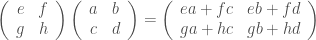
These numbers look familiar, don’t they?

In fact, the diagrams that we have been drawing all along are actually in 1-1 correspondence with matrices that have natural number entries. Moreover, just as composition of diagrams with one dangling wire at each end corresponds to multiplication of natural numbers, composing diagrams of arbitrary shape can be understood as matrix multiplication. We will go through this in more detail next time.

For now, a quick summary: the diagram

corresponds to the matrix $\left(\begin{array}{cc} a & b \\ c & d\end{array}\right)$ . In general, the number of columns of the corresponding matrix is the number of dangling wires on the left, and the number of rows is the number of dangling wires on the right. Moreover, the entry at row i and column j is the number of paths from the jth wire on the left to the ith wire on the right.

Finally, the composition

corresponds to the matrix obtained by performing the matrix multiplication ①.

And, as you’ve seen, it all follows from how adding and copying interact!

Continue reading with Episode 11 – From Diagrams to Matrices

9. Natural numbers, diagrammatically

We spent the last few episodes assembling our toolbox of equations. The game in graphical linear algebra is as follows: we consider two diagrams to be equal exactly when we can use the equations and graphical reasoning to prove it. If we cannot, we will consider them to be different. A mathematician would say that we are considering the free system on this set of equations.

If this idea is not clear, then imagine playing a board game: the things that you are allowed to do are only those that are specified in the rules. If something is not in the rules, then it is not allowed. Board game rulebooks typically do not include every possible way of how one could break the rules. People are way too creative at cheating; no wonder that law is such a complicated mess! In a similar way, we are usually not going to explicitly say when two diagrams are different: we consider them to be different if it is not possible to show, using the rules, that they are equal.

Anyway, here’s a convenient cheat sheet for the equations we have met so far, to save unnecessary clicking between episodes.

I hinted back in Episode 3 that graphical linear algebra has something to say about counting. That’s the plan for today. We will focus our attention on a very particular class of diagrams: those with exactly one dangling wire on the left and on the right. As it turns out, such diagrams are very closely related to natural numbers: that is, non-negative integers 0, 1, 2 and so on. For example it makes a lot of sense to associate the following diagrams with the corresponding numbers:

Remember the intuition about numbers travelling on wires? Well, associating numbers to diagrams is compatible with all that. For example, let’s consider sending a number x on the left dangling wire of the diagram that we are associating with the number 3.

The output is x + x + x = 3x. So, whatever the input, the diagram acts by multiplying it by 3. If you look at the diagrams for 0, 1 and 2, the idea is the same.

There is also a nice graphical intuition at play here: the number associated to a diagram is the number of paths from the dangling point on the left to the dangling point on the right. So, in the diagram to 0 there are no paths from left to right, in 2 there are two different paths, and so on. This graphical intuition is very important and we will come back to it again soon.

Although this is all quite cute, the correspondence between numbers and diagrams is not merely skin deep. As we will discover, the algebra of diagrams allows us to perform the basic operations of arithmetic: addition and multiplication. Thus, while our slogan so far is that linear algebra is all about what happens when adding and copying meet, we can actually be more extreme: even the basic idea of natural numbers is explained by adding and copying!

We start by defining a translation from numbers to diagrams, which will be useful for us as a syntactic sugar. The expression “syntactic sugar” is probably quite familiar to you if you are a programmer: it means a construction that is useful to have as part of your language, but that does not actually add anything new: the language does not become any more expressive. Syntactic sugar can always be translated away to phrases that we had before, but having it may be convenient for several reasons. This is exactly the case that we have before us.

Our syntactic sugar is a family of special diagram components, one for each natural number. We start with our good friend 0. We use the special := notation to indicate that we are actually defining the thing to the left in terms of things that we already know about.

The reason for the name (base) is that we will define the syntactic sugar recursively, and the definition above is the base case of the recursion. The recursive case is:

Maybe you have not seen the use of recursion before. It is something that many first year Computer Science undergraduates are very scared of; I know from personal experience! The reason is that, if you look at (rec), we are trying to define something (the left hand side), but we are using it again in the definition (the right hand side). This looks circular and weird — but don’t worry, it makes sense, and is not very difficult. The best way to get the hang of it is to experiment with some concrete examples.

So let’s understand the first few numbers, starting with 1.

We use (rec) to get the first equality, then (base), then (Unit), then (Counit). So the diagram that corresponds to 1 is simply the identity.

Let’s do 3 now.

We use (rec), then (rec) again, and then we use our knowledge of the diagram for 1, which as we have discovered above, is simply the identity.

It is important not to confuse the syntactic sugar for a natural number with a number travelling on the wire, as per our standard intuition. In fact, the sugar acts by multiplying its input by the number it represents, like so:

Let’s prove this!

But how does one prove something about all natural numbers? We could start showing that it holds for individual cases, say n = 13, but that would not be very satisfactory. Maybe we got lucky with that particular choice, maybe it’s not true for n = 12?

The trick is to use mathematical induction: if we show that the above is true for n = 0 (the base case) and whenever it is true for n = k then it is also true for n = k + 1 (the inductive step), then we can conclude that it holds for all natural numbers n. It’s kind of a bootstrapping process: how do I know that it’s true for n = 13492? Well, we know it’s true for n = 0. But because it’s true for n = 0, it must be true for n = 1, using the inductive step. But because it’s true for n = 1, it must be true for n = 2. And so on, until eventually we get to n = 13492.

We start with the base case, n = 0. Using (base) we need to check the behaviour of the following circuit.

And indeed, according to our established intuition about how the generators behave, a number x arrives on the left, is discarded, and a 0 is produced by the zero generator. But 0 = 0x, so the effect of the 0 sugar is to multiply its input by 0, as we are claiming.

Now let’s assume that this works as advertised for n = k and try to show that it holds for n = k + 1. The assumption is called the inductive hypothesis. For the k + 1 circuit, we use its defining equation (rec) and consider the behaviour of the following.

Again a number x arrives on the left, and is copied. The first copy is fed into the k sugar, which, by the inductive hypothesis, multiplies its input by k, resulting in the output kx. The second copy of x is untouched, and so kx and x are fed into addition, resulting in the output kx + x. But kx + x = (k + 1)x, which is what we want!

This concludes the induction and the proof. We will do many more induction proofs, so if all this is new to you then you will have plenty of examples to get comfortable!

We now move to the meat of this episode: showing how the algebra of diagrams can be used to express some familiar operations on numbers. Let’s start with adding: we willl prove that the following equality holds for all natural numbers m, n:

One way of understanding (sum) is that it show that ordinary, old-fashioned addition of natural numbers is already a part of our language: we can understand it with the basic operations of graphical linear algebra.

So let’s start by looking at what happens when n = 0, the base case of the induction.

We first use (base), then (Unit) and (Counit) together in a single step. Finally m = m + 0, as we all know. This shows that, no matter what m is, (sum) is true when n = 0.

Next, let’s look at the inductive step: remember, we can assume that what we want to prove, (sum), is true whenever n = k, and simply show that it is true for n = k + 1. Here we go:

First we use (rec), then (Assoc), then (CoAssoc). Next comes the use of our inductive hypothesis, and finally we use (rec) again. This completes the induction, and the proof of (sum).

We are going to prove a few more things in this episode. The first is the following useful equation, which holds for any number m.

Again the proof is by induction. For m = 0, it suffices to use (B4), the bone equation.

Next the inductive step.

First we use (rec), then (B2), then the inductive hypothesis, and finally (Counit). That’s (discarding) proved then.

The next property that we need is the following.

Let’s do the induction. For the base case, we have:

The proof of the inductive step is long, but not very complicated. We just need to apply (CoAssoc) a number of times and (CoComm) once to get the right alignment of the copies on the left. In the third step we use the inductive hypothesis. It is not super important to follow all the steps, so feel free to skip it.

If you did go through the proof carefully, maybe you spotted the one step where I cheated. It was the point at which I used (sliding) — remember that we are allowed to slide generators along wires. The reason why I was being slightly naughty is that the diagram for the number k is not, strictly speaking, a generator: it is syntactic sugar. However, because it is built from basic generators, one can show without too much difficulties that it can also be slid. In fact, it is not too difficult to show that any diagram whatsoever can be slid along wires.

Here’s a claim which I will not prove, because you have seen enough of examples of how to prove things by induction to be able to do it yourself. The claim is this:

For any natural number n, the bizarro version of the diagram for n is itself.

This is a useful fact to note, because we immediately get the following two things for free:

The reason why we know that (zero) and (adding) hold is because they are the bizarro versions of (discarding) and (copying). We can simply repeat each step in the proofs of (discarding) and (copying), but in the bizarro world.

We should spend a little bit of time discussing (adding), because it seems contrary to our expectation that the adding generator ought to be adding things. So why isn’t m + m = 2m? Well, let’s come back to our intuition of numbers on wires. Consider the left hand side of (adding), it has two dangling wires on the left on which we can send two numbers x and y. Next, remember from the introduction that the diagram for m acts by multiplying its input by m. Then the two outputs are fed into the adding operation, like so:

What about the right hand side? Performing the individual operations gives us the following behaviour:

But multiplication distributes over addition, so m(x + y) = mx + my; the behaviour of the two sides of (adding) is the same. We have, of course, already seen how to add natural numbers in graphical linear algebra, and it is handled by a combination of the adding and copying generators, as demonstrated in (sum).

There is just one more thing to prove in this episode, and it concerns another famous operation on natural numbers.

Just like (sum) can be understood as saying that ordinary addition of natural numbers can expressed using graphical linear algebra, (multiplication) is saying that ordinary multiplication of natural numbers is just composition.

To prove it—you guessed it!—we will use induction. The base case is the following, and we have the chance to use the (zero) property.

Next comes the inductive step, where we use both (adding) and (sum).

This completes the proof of (multiplication).

We have shown how natural numbers, addition and multiplication arise in graphical linear algebra. But there is one point about which you may be nervous: we have shown all kinds of useful properties, but what if actually 2 = 3 in graphical linear algebra? What if every number is equal to every other number? Maybe there is some crazy graphical proof that shows this? And how do we show that one cannot prove something, anyway? This is where the graphical intuition about counting paths comes in, and we will come back to this in the next episode.

Another question that you may have is the following. We have shown that all natural numbers can be understood as certain diagrams with one dangling wire on the left and one on the right. But are there some diagrams of this kind which are not equal to one that represents a natural number? In fact, this is not the case: this class of diagrams is in 1-1 correspondence with the natural numbers: every diagram with one dangling wire on the left and right is equal to one that comes from a number. There are several ways to show this, and we will explore some of these techniques in subsequent episodes.

Continue reading with Episode 10 – Paths and Matrices

8. When Adding met Copying…

Let’s start with a recap. Last time I claimed that linear algebra was all about what happens when adding and copying interact. So far, though, we have only focussed on properties satisfied by adding and copying in isolation. Properties such as (Comm) and (CoComm).

We noticed that adding and copying are bizarro version of the other: not only in the way that they look, but also in the equations that they satisfy. Remember that the word bizarro, as we have been using it, means to reflect the diagram and invert the colours. Left switches places with right, and white switches places with black.

In this episode, copying meets adding for the first time. Sparks fly.

It’s time to meet one of the most interesting equations of graphical linear algebra.

Equation (B1) is by far the most complicated of the ones that we have seen so far, so let’s stop for a moment and take the time to understand and appreciate it. First, notice that both the left hand side and the right hand side have the same number of dangling wires on both sides: two on the left and two on the right. Remember that it is important that any equation that we write down satisfies this property: otherwise the compositionality property—that is, swapping diagrams for equal diagrams in some larger context—wouldn’t make any sense since we wouldn’t know what to do with the extra/missing wires!

Next, let’s try to convince ourselves that (B1) makes sense by using the intuition of numbers moving along wires. In the left hand side, there are two dangling wires on which we can input numbers x and y, and they are first added, then copied. Like so:

Now let’s do the same thing for the right hand side: first we copy the two numbers, we swap two copies in the middle, then we add. Like this:

Since we are making no assumptions about what actual numbers x and y represent, our demonstration shows that the behaviour of the left hand and the right hand sides of (B1) is the same: we can’t detect any difference between them if we cover up the internal contents of the circuits and only experiment with them by providing various inputs and observing outputs.

I want to say one more thing about (B1) — its bizarro version is itself! If we reflect the left hand side and switch the colours, we get the left hand side again. Same with the right hand side. By the way, here’s a useful exercise for you to get comfortable with the algebra of diagrams: write down a formula that constructs the right hand side of (B1) using the operations ⊕ and ; on the basic generators, identity and twist. Remember how we did it for Crema di Mascarpone?

What happens when adding meets discard, copy’s sidekick? That scenario gives rise to the second key equation.

The rationale for (B2) is easy: in the left hand side, we add our two inputs and then throw away the answer. But, clearly, the observable behaviour is the same if we just went ahead and threw away the two inputs without adding: the behaviour in both cases consists of taking any two numbers and not producing any results.

Next up is an equation that concerns the situation when zero meets copying.

Remember that the behaviour of the zero generator is simply to output the number 0 on its result wire. If I copy 0, I get two 0s. That’s what (B3) is saying.

Take another look at (B2) and (B3). Can you see how they are related? One is the bizarro version of the other. Graphical linear algebra is full of bizarro situations like this: we already noticed that the equations for adding and copying are bizarro versions of each other. In fact, this is part of a general fact of graphical linear algebra:

If an equation holds, then its bizarro version holds too.

This will be true for the entire run of our story; even as we consider additional generators, diagrams and equations. It’s a useful thing to keep in mind because sometimes it will save us half the work, and sometimes it will allow us to see connections between seemingly quite different phenomena.

This is probably a good point to take a short break for a discussion about our methodology. Some of you, probably including most of the non-mathematicians, may be confused as to why we keep identifying certain equations and giving them names.

I hinted a few of episodes ago that we want to gradually get away from thinking about “numbers moving on wires”. Instead, we will use the key equations that we have identified so far as axioms; that is, basic postulates that we simply accept to be true.

Much of our attention will be on examining what kind of things these axioms allow us to prove, and what they do not prove, using only the rules of working with diagrams together with basic logical reasoning. Just as when we proved the upside down version of (Unit). Historically, this kind of methodology—that is, identifying basic properties and seeing how far they get you—is tried and true: the tradition goes back at least to 300 BC with Euclid and his elements.

In this episode we identify four equations; we have seen three of them so far, (B1), (B2) and (B3). Together with the three equations for adding and the three for copying, this system of ten axioms will suffice for the next few episodes. As we will discover, it is already a very interesting system, even if it may not look like much at this point! For example, we will use diagrams to do some basic arithmetic in the next episode.

The final axiom is a bit strange.

First, the left hand side is what happens when you compose zero with discard. It’s a strange kind of diagram that we have not seen before, because there are no dangling wires at all. But what is the right hand side? I didn’t forget to draw it: it is also a diagram, the diagram with nothing in it. A blank piece of paper.

We will sometimes call the left hand side of (B4) by the extremely technical name “bone“. I guess that I probably don’t need to explain the etymology. The name was invented by my coauthor Fabio—at one point the whiteboard in my office was covered with them and we needed to call them something!

So (B4) tells us that, in any graphical proof, whenever we come across a bone we can simply erase it. That’s because, if I output zero and promptly discard it, it’s like doing nothing at all.

Mathematicians call structures that satisfy equations (B1) through to (B4) with different names, typically bimonoids or bialgebras. We will use the term bialgebra. It’s not a great name, but it will do.

There is one more thing to be said. Maybe you remember that, in ordinary arithmetic, products distribute over additions: so the following is true for any numbers a, b and c:

a(b+c) = ab + ac

In the equation above, when evaluating the left hand side, the addition comes first followed by a multiplication. Instead, in the right hand side, the order is reversed: we multiply first and add later. So the distributivity property reversed the order in which we perform operations.

Our new equations from this episode can also be understood as reversing the order of the operations. For example, take another look at (B1). In the left hand side, the addition comes first followed by a copy, while in the right hand side it is the copying that comes first, followed by additions.

In fact, it is really the case the equations (B1) through to (B4) can also be considered as a distributive law in a formal mathematical sense. I will not go into the details of this now, because it is not strictly necessary to understand in order for us to make progress in the story. For the interested, it is all explained in a wonderful paper by Steve Lack. Steve is one of the extremely brilliant category theorists that I have been lucky enough to meet and learn from: he supervised my honours project at Sydney Uni, back when I was finishing my undergraduate degree.

Continue reading with Episode 9 – Natural numbers, diagrammatically

7. Copying, Discarding and The Slogan

Graphical linear algebra has five stars as its leading actors. We know two of them already: addition and its trusty sidekick zero. Two more make an appearance in this episode: their names are copy and its sidekick discard. We will have to wait a few episodes for the fifth star to make an appearance. Sometimes our main stars will have to play in the mirror; you will see what I mean when we get to that point in the story. There is also a supporting cast, by the way. We will them meet in due course, but they are nowhere near as important as the five central players.

In the Real World™, the ability to copy and discard things seems to be quite rare. When making Crema di Mascarpone, following our recipe from last time, it is not enough to just have one egg. We can’t just magically copy it. Also, after cracking the egg, you are also left with some eggshells. Unfortunately, I omitted this from the—therefore somewhat unrealistic—recipe, and this mistake was duly pointed out in the comments section. Even if you do throw the shells in the bin, they don’t just magically disappear.

Of course, one thing that can be copied is (the non quantum kind of) information. For example, a file on your hard disk can be copied and deleted as many times as your disk space will allow. Copying and discarding is the main topic in this episode. So without further ado, it’s time to meet the new generators.

First, the copy generator. It has one dangling wire on the left, and two dangling wires on the right, just like Crack Egg generator from the last episode. We will draw it with a black filled-in circle, so that we don’t confuse it with adding.

We will continue to use our intuition of numbers travelling from left to right along wires for now. Copy takes one argument and has two results, and it lives up to its name by—wait for it—copying. For example, if a 42 arrives as an argument, two copies of 42 exit as results. Like so:

Copy works the same way for any number that arrives as its argument, so we could summarise this behaviour by using a variable.

That’s about all there is to say—copy does what it says on the tin. It’s not complicated.

So what about its sidekick, discard? It also gets a generator, with one dangling wire on the left and no dangling wires on the right.

Discard, again as its name implies, simply throws away anything supplied as its argument. Simple enough — a 42 may arrive, and it is forgotten. Think of discard as an efficient number disposal system.

There is an interesting thing to notice about copy and discard; they look like adding and zero, but reflected, as if a mirror were placed on the side. More accurately, a special “colour inversion” mirror that turns white into black and black into white. What I mean is that, while add has two dangling wires on the left and one on the right, copy has two dangling wires on the right and one on the left. Zero and discard are, similarly, reflections of the other.

Another interesting fact is that copy and discard satisfy three equations that are very similar to the ones that we already met for adding and zero. We will run through them now.

First, there is the (CoComm) rule. If I copy a number then its the same thing as copying that number and swapping the copies. It’s obvious right? The copies are exactly the same, so I can’t tell which one is which: the behaviour of the left hand side and the right hand side is the same.

By the way, I should explain the “Co” in front of “Comm” in “CoComm”. Mathematicians often use the “co-” prefix to talk about familiar things that have been turned around. And (CoComm) is just (Comm) reflected and coloured black.

Next up is (CoAssoc), which is the reflected, photographic negative copy of (Assoc). If we copy something and then copy one of the copies again, then we have three equal copies. It doesn’t matter which of the two initial copies we copy again.

Finally, I have (CoUnit), which is the bizarro version of (Unit) (for the non-nerds amongst you, the bizarro world is a strange “reverse” version of Earth in the Superman universe where cigarette butts are treasures, evil is good, and so on). Again (Counit) is easy to understand: if I copy something and throw away one of the copies, it’s as if I have done nothing at all.

By the way, mathematicians sometimes call a structure that satisfies (CoComm), (CoAssoc) and (Counit) by the rather grotesque name cocommutative comonoid. And because the word “cocommutative” sounds like it has something to do with mutant coconuts, we will just say commutative comonoid. Copy and discard are, therefore, an example of a commutative comonoid.

Remember the upside-down (Unit) law that we proved last time? Here is its bizarro version.

Look again at the diagrammatic proof at the end of the last episode. We can use exactly the same steps, but in the mirror, using (CoComm) and (CoUnit) instead of (Comm) and (Unit). Take a break from reading now, grab some paper and a pencil, and draw the steps!

In fact, any diagrammatic proof about addition that uses only (Comm), (Assoc) and (Unit) can be reflected to give us a similar proof about copy and discard. This can potentially save a lot of work when proving things: we already know that the upside-down version of (Counit) is true because we proved the reflected version.

Mathematics in general, and especially category theory, is full of situations like this, which are often called dualities. In a duality, you prove one thing and you already know that its backwards version is true. This is because the two proofs are morally the same thing, one is just the bizarro version of the other.

It’s time for the first big reveal of the story. We have talked about the ways in which we can understand adding and copying numbers with diagrams. Linear algebra is all about adding and copying. Here is a nice, bold slogan:

Linear algebra is the mathematics of adding and copying.

By the way, I mean adding and copying together with their respective sidekicks, zero and discard. And I mean what the slogan claims quite literally: if you already know about linear algebra, then every concept you learned is a consequence of the very beautiful ways that adding and copying work together. Matrices, spaces, bases, eigenvalues, eigenvectors, and so on. If it’s a concept of linear algebra, it concerns some interesting interaction between adding and copying. It turns out, probably not surprisingly, that adding and copying are quite common in many areas of science and mathematics: hence the Makélélé status of linear algebra.

Why is it, then, that linear algebra is not usually taught as the thing that happens when addition meets copying? I think that it is because traditional mathematical notation is not well suited for expressing the operations of copying and discarding in isolation. I can write 2 + 4 and everyone knows that I am adding two numbers. But how do I express the action “copy 2” or “discard 5“? This is not a problem for our graphical notation: addition and copying have equal status as generators. One is not any more awkward to talk about than the other.

As a consequence, the graphical language that we are using is perfect for showing off the inner beauty of linear algebra. Similarly, it is more directly related to several of linear algebra’s glamorous applications than traditional notation. You will see what I mean if you stick around. Copying meets adding for the first time in the next episode.

Continue reading with Episode 8 – When Adding met Copying…

6. Crema di Mascarpone and Diagrammatic Reasoning

First an announcement. Graphical linear algebra is going on the road!

I will give a tutorial on it at QPL 2015 in Oxford on 13-14 July.

I will also talk about it at the ICTAC summer school, in Cali, Colombia, on 25-27 October. I’ve never been to Colombia before, I’m super excited!

In this episode we are going to discuss the recipe for Crema di Mascarpone, one of my favourite desserts. We are also going to write our first proof, using only diagrams.

First, a recap of where we are in the story.

We have been talking about addition and zero, and how to construct diagrams. Addition and zero are two generators (basic diagrams) of our system:

We can make more complicated diagrams with two operations: direct sum (⊕) and composition (;). Direct sum stacks its arguments one on top of the other, and composition connects wires.

When constructing diagrams we also often use two special diagrams, called identity and twist.

Identity and twist are the basic plumbing of diagrams; they give us some flexibility, allowing us to connect the right “studs” to the right “holes”, to use a Lego analogy.

Let’s leave addition and zero for now, and move on to sweeter things.

Crema di Mascarpone is the delicious, silky smooth filling that you find inside Tiramisù. It’s also great as topping on Pandoro or Panettone, the two famous Italian christmas cakes. A word of warning to those planning to visit Italy: it may be the case that it’s a minor misdemeanour to put Crema di Mascarpone on a Panettone; I believe that it’s only officially sanctioned on a Pandoro. Nevertheless, this crime is of course nowhere near as severe of drinking a cappuccino after 11am or (the horror!) putting pineapple on a pizza. Apologies to my Italian readers for making you even consider the possibility of such an atrocity.

You will need two eggs, 200g of Mascarpone and 2 tablespoons of white sugar. We will represent the recipe for Crema di Mascarpone as a diagram, but since making food is much more complicated than addition, we first need to introduce a whole load of generators:

Of all of these, we should stop and examine the first—the Crack Egg generator—because it’s the only one we have seen so far where there is more than one result wire. We will meet a generator like this in the next episode. It’s a very important part of the story of graphical linear algebra.

The rules for direct sum and composition are a little bit more complicated than the ones we have already seen, because it is not enough to know just the number of dangling wires but also what the wires represent. We don’t want to confuse our ingredients! We would also need a few different versions of identity and twist to give us the plumbing for all the different kinds of wires: for instance we need the identity wire for mascarpone, and a twist where a yolk and white wires cross over, and so on. Since this blog is not really about recipes, we are going to cheat slightly and not going to bother writing down the more complicated versions of the rules, nor the more complicated plumbing. Let’s keep things simple.

Here is the recipe for Crema di Mascarpone.

We could write a formula for this, even if it’s not as nice to look at as the diagram.

(C ⊕ C ⊕ id₂) ; (id ⊕ tw ⊕ id₃) ; (W ⊕ B ⊕ id) ; (id ⊕ S) ; F

In the formula C stands for “Crack Egg”, W for “Whisk”, B for “Beat”, S for “Stir” and F for “Fold”. We also use id to stand for identity and tw for twist. Finally, id₂ and id₃ stand for, respectively, the direct sum of two and three identity wires.

It’s maybe not clear how to pass from the diagram to the formula. So let’s develop a technique for this. First, I choose appropriate points to divide the diagram into vertical slices.

If I name the slices V, W, X, Y and Z, then it’s clear that the whole diagram can be constructed by evaluating

V ; W ; X ; Y ; Z

It is important to keep in mind that the composition operation on diagrams is associative: whenever I have diagrams X, Y and Z that can be composed, then (X ; Y) ; Z is the same diagram as X ; (Y ; Z). For this reason it makes sense not to write parentheses in the equation above — the order in which we perform the compositions does not matter!

The final vertical slice, Z, is easy: it’s just the Fold generator. We now divide the remaining vertical slices horizontally, so that each of the resulting rectangles is either a generator or basic plumbing. Like so:

Now, scanning down each slice we can write down an expression for each of V, W and so on. For example

V = C ⊕ C ⊕ id ⊕ id.

We again left out parentheses, because—you guessed it!—direct sum is associative.

That’s how we can get to the long formula for the recipe: first subdivide into vertical slices, then subdivide those slices horizontally. Now, while Crema di Mascarpone is amazingly delicious, the real point of this section is to describe how to work with diagrams. There are four rules to remember. The first is:

Rule 1: Always draw diagrams so that it’s possible to subdivide them, obtaining a formula that uses the generators, plumbing, ⊕ and ;.

So here’s an example of something that we are not allowed to draw at the moment.

Let’s examine why. It would make sense to draw the vertical bars around addition, since we know it’s a generator. We get something like this.

So far so good: the middle slice is identity direct summed with addition. But what are we to make of the left and the right slices? It looks like we would need some plumbing that looks like

and

The first one has no dangling wires on the left and two on the right, and the second two on the left and none on the right. But we don’t have any advanced plumbing like this, we only have a supply of identities and twists in our toolbox. Something has gone wrong — by Rule 1 this is not a diagram that we are allowed to draw.

The diagram that we disowned is actually quite interesting: the result of the addition is “fed back” as the first argument. Feedback is extremely important in computer science, control theory and engineering. It has launched a thousand papers. Graphical linear algebra has some interesting things to say about feedback too, as we will see.

Rule 2: Wires don’t tangle

This rule tells us about how the plumbing in our diagrams behaves. For example, we consider the following two diagrams to be equal.

There is an intuitive way to think about the equality above: imagine starting with the left hand side and pulling on the wires until they are tight. Since we are in the beautiful world of graphical linear algebra and not in the hideous world of the back of your TV, the wires do not get tangled. We end up with the diagram on the right hand side.

Here’s a more complicated example, but the same intuitive principle applies (although, in the underlying mathematics, the equations hold for different reasons).

The thing to keep in mind is that in wiring, i.e. the kinds of diagrams that we can construct with just the identity and the twist, what matters is which dangling positions on the left are connected to which dangling positions on the right. By the way, we can understand these kinds of wiring diagrams as encoding permutations, and—long story short—composing wiring diagrams works the same way as composing permutations.

Rule 3: Generators can slide along wires

There are two things to say here. Let’s start by thinking about the part of the recipe where we crack the eggs.

It makes sense to think about the horizontal axis of the diagram as time, so in essence, our recipe says that we should crack our two eggs simultaneously. Fortunately, graphical linear algebra understands that you only have two hands. The following diagram is considered to be equal.

Here we cracked the first egg before we cracked the second. But also the following diagram is considered equal.

So it does not matter in which order we crack the eggs, as one would reasonably expect when preparing desserts. We can move between the three diagrams by sliding the generators along wires. This kind of action is always allowed, and it won’t change the meaning of our diagrams.

There is a second way in which generators can slide along wires, and it involves the twist. Suppose that, in some hypothetical dessert, we had to whisk some egg whites, but we also had to crack an egg for some other purposes. Also, it turned out that our ingredients were in the wrong order on the table, so we had to rearrange them.

In this situation, we can slide the Crack Egg generator along the wires to the right, past the twists, like so.

So, essentially, we can wait with the cracking of the egg until we finish the whisking, and just rearrange the egg and the whisked egg white on our ingredient table beforehand. Look at the two diagrams above and imagine the Crack Egg generator sliding from its position in the first diagram to its position in the second diagram. Simple!

Rule 4: Diagrams are compositional

Compositionality is something that many mathematicians take for granted. They sometimes they call this principle “substituting equals for equals”. What it means is that in an algebraic structure, once you know that two things are equal then you can swap them as you like in larger formulas, and the two formulas will still evaluate to equal results. For example, we can calculate that 1 + 3 = 2 + 2. Next, we can use this fact to not actually do the following calculation. We can be lazy, because we already know it’s going to be true!

(1 + 3) × 4134221=(2 + 2) × 4134221

We can obtain the right hand side from the left hand side by replacing 1 + 3 with something equal to it, 2 + 2. Compositionality says that the results will be equal.

The real world is, alas, much more complicated. Let’s discuss one example that’s close to my heart. When I was a teenager, computers doubled their speed every 18 months or so. This is because engineers were able to fit in many more, smaller transistors on chips, and this made it possible to increase the clock speed; the pulse that determines how fast computers make their calculations. Engineers are still able to make smaller transistors and put more of them on chips. Unfortunately, because of the underlying physics, they are not able to ramp up the clock speed any more. When computer companies sell you their machines now, they no longer focus on the clock speed so much; instead they tell you about how many cores their computers feature. Dual core, quad core, hex core, etc. The more cores the better. If you have a mobile phone then you are probably carrying several hundred cores in your pocket. So what is a core exactly?

A core is a processing unit. Having two cores typically means that your computer is able to do two things at the same time. If you have hex core then it should be able to do 16 things at the same time. Sounds great, right? Well, the problem is that nobody told the programmers how exactly to take advantage of extra parallelism. Writing concurrent programs is hard.

I think that one reason why concurrency is hard is because the tools that we give to the programmers are not compositional. Two programs might have the same behaviour if we think of them as running on one core, but they may act very differently if ran in parallel with another program. This is because of things called race conditions. It is really, really difficult to understand non-compositional things.

Of course, I’m over simplifying things in this brief explanation; concurrent programming is a huge area. But maybe I will come back to this topic at some point in the blog. I have some work in progress, based on the ideas of graphical linear algebra, that may be helpful.

Let’s get back on topic: the good news is that diagrams are compositional. If we know that two diagrams are equal then we can substitute them for each other in more complicated diagrams. This is one of the principles of diagrammatic reasoning: writing proofs with diagrams. We will work through an example below.

The four rules cover all you need to know about diagrams in order to do graphical linear algebra. You may be wondering why does it all work; where do the rules come from? The answer is that the diagrams, which many people call string diagrams, are actually a very nice notation for elements of mathematical structures called PROPs (which stands for product and permutation categories, somehow). PROPs are, in turn, examples of mathematical structures called symmetric monoidal categories. It is not important, at the moment, to delve into their arcane lore. Instead, keeping rules 1-4 in mind, we can start having fun.

Let’s use this knowledge to write our first completely diagrammatic proof.

Remember that, so far, we have identified three equations.

Now we are going to prove that the following is true.

We will use only our chosen three equations, and the principles of diagrams that we discussed earlier. Since it’s our first proof, we will go slowly; eventually, when you are more comfortable with the ideas, we will be able to speed up quite a bit.

Let’s start with the left hand side. First, draw a red square around the addition generator. The red square is not really a part of the diagram, it’s only there to help us to focus. The addition generator is the left hand side of (Comm), so using the principle of compositionality, we can replace everything inside the red square with the contents of the right hand side of (Comm).

Now, we can slide the zero generator across the twist. Here we are using the principle of sliding generators along wires.

But this is just the left hand side of (Unit). So we can replace it with its right hand side.

And we’re done; we have followed a chain of reasoning that took us from the left hand side to the right hand side of the equation that we were interested in. Actually, it turns out that we didn’t need to use (Assoc) at all in the proof.

Cool, huh?

Continue reading with Episode 7 – Copying, Discarding and The Slogan.

5. Spoilers, Adding (Part 2) and Zero

Several people have asked for motivation to keep reading. “What will I learn if I stick around until Episode 10, or Episode 20?” It’s understandable: it takes effort to read this stuff, and you don’t want to waste your time.

I don’t want to give away the plot twists ahead. The thing about plot twists is that you only appreciate them fully if you are engrossed in the story. What if I told you about the events of the Red Wedding at the start of season one of the Game of Thrones? You wouldn’t have reacted like this!

Having said that, if you are dying of curiosity and you absolutely must know now, then there is a paper full of spoilers on the About page. For the people who just want to be teased, the next few paragraphs are a brief trailer for approximately the next 15 episodes. If you don’t know the jargon of linear algebra, don’t worry if you don’t understand; I will explain the terms when we need them. Feel free to skip to today’s content, below the horizontal line.

In the next 5 episodes you will learn how to do diagrammatic proofs, and how certain kinds of diagrams capture the same information as matrices. You will understand matrix multiplication in a way that you probably have never seen before. The 10 episodes after that is the really exciting stuff.

In ordinary linear algebra, the one taught in first year undergraduate maths around the world, there comes a point in the exposition where there is a certain sleight of hand, where your lecturer pulls a rabbit out of a hat, so to speak. It typically comes just after you learn about the algebra of matrices and vectors. Suddenly you’re talking about vector spaces and subspaces, which are sets of vectors closed under addition and scalar multiplication. Where did the sets of things come from?

In graphical linear algebra we will not need to leave the pleasant world of diagrams. We will not need to talk about sets of things. The conceptual leap from matrices to spaces in graphical linear algebra is, in my opinion, simply wonderful. I am very proud to have been involved in its discovery. It will be one of the highlights of this story, and will also have several side-effects. One will be a graphical way of understanding fractions, which includes a rather unexpected bombshell featuring the star of this episode, zero. Stay tuned!

Diagrams are very much like magic Lego from the last episode. Remember how the important thing with magic Lego was keeping track of the number of holes on the left and the number of studs on the right? Diagrams are similarly easy: we only need to record the number of dangling wires. Here’s the diagram for addition that we discussed two episodes ago, together with the associated information (2,1) that tells us that there are two dangling wires on the left, and one dangling wire on the right.In graphical linear algebra, this diagram is considered a basic, atomic diagram, just like the basic bricks of magic Lego. We will construct more complicated diagrams from it and other “core” diagrams. Instead of saying “basic diagram”, we will use the word generator from now on.

There are two very special diagrams that it’s high time we met. We will see why they are special in the next episode, which will wrap up the Rules of the Game of graphical linear algebra. The first one may seem a bit useless. You will learn to love it though, because it’s more important than its rather unassuming looks. In fact, it has a name of its own, it is called identity. Identity is simply a single wire that dangles from both ends. The second special diagram also has a name—it is called twist—and consists of two crossing wires, dangling from both ends. The algebra of diagrams uses the same operations that we used for Lego. Actually, we can use exactly the same rules. Direct sum of diagrams works just like we would expect: we stack the first argument on top of the second. Why did the identity become curved in the second diagram? Well, there’s no reason for it not to curve. I could have drawn it straight, and we would have considered that result to be the same diagram. Just like magic Lego, where we deformed the shapes of the bricks as if they were rubber, we can deform diagrams. When deforming diagrams, we will usually leave the circles alone, and simply stretch the wires, as if they were rubber bands.

To get back to the concrete operation above, we just have to draw the identity wire below the addition in the result. No rulers needed! The important information in a diagram is what connects to what, reading from left to right, and in which order the generators (basic diagrams) come, reading from top to bottom. For now, that’s all you really need to know; in the next episode we will discuss the kinds of things that you are not allowed to do with diagrams.

Just like in Lego, direct sum is not commutative. Now let’s focus on composition, which also uses exactly the same rule as in the last episode. In Lego, composition worked by fitting studs into holes. In diagrams, we simply connect wires together. For example: You’ve already seen the result above, it is the right hand side of (Comm) equation from two episodes ago! Here is that equation again, for your convenience. Composition is easy, right? Now let’s construct some other interesting diagrams: and This brings us to the second equation of graphical linear algebra. Can you guess what it means? Think about it for a few moments before reading on.

(Assoc) captures the associativity property of addition. Let’s try to figure out what it says and why it makes sense. Consider the left hand side, and think about variables x, y and z arriving on the dangling wires from the left: x on the topmost, then y on the middle and z on the bottom wire. In the left diagram, the first thing that happens is that we add x and y, and then we add z to the result. Like this: Doing the same thing on the right hand side gives us: An operation is associative when it doesn’t matter how you bracket it; the result will always be the same. Addition is a well-known example of an associative operation. A mathematician might write:

∀ x,y,z. (x + y) + z = x + (y + z).

That is, no matter what numbers we substitute x, y and z, it does not matter whether you first calculate x + y or y + z.

Covering up both sides of (Assoc) with a square piece of paper of the right size gives us two diagrams that both look as follows

and—using the associativity property of addition—no matter what three numbers we feed in along the wires on the left, the result will be the same. In other words, the two diagrams in (Assoc) have the same behaviour.

It’s time for the star of this episode to make its entrance.

Zero is absolutely essential in linear algebra. It is a mathematical abstraction, and one of the first ones we learn at school. For that reason, zero may seem to be quite obvious to you now. In fact, it was a major discovery in the history of science, and it is far from trivial. How can we tell that, one, zero is very important, and two, that it wasn’t so obvious to discover?

Some good evidence for these claims is, one, we all know what it is, and two, that in the entire history of human civilisation, it was only discovered twice, maybe three times.

If something is easy and useful, it tends to be invented many times. For example, it’s a fairly simple observation that when a tree falls in a body of water, it tends to float. A canoe is only a few thoughts away. So canoes are easy to conceive of, and are clearly very useful. For those reasons, they were invented and reinvented many times, in many different places across the globe over the last few millenia.

If something is hard and useless, it tends to be invented in academic departments across the world, and be understood by very few, very specialised scientists. I will not give you any examples, dear reader, because I live in a glass house and I certainly don’t want to start throwing stones. I don’t think that hard and useless is an insult by the way; let me explain why. Hard and useless things sometimes lead to hard and useful things. This is why the hard and useless is worth doing.

If something is hard and useful—the most interesting of cases—it tends to be invented a small number of times, and the idea spreads quickly from person to person, from culture to culture. Zero is firmly in this category. Hard and useful things are very rare. Nowadays, they are usually called scientific breakthroughs.

There has been intense political pressure on the academy to stop working on hard and useless things over the last 30 years or so. The result is a new generation of academics who do easy and useful things, things that impact the economy in the 5-10 year scale, and which bring in research funding. This is by design, because research funding is closely tied to academic career progression. Unfortunately, it’s not very hard to disguise easy and useless things as easy and useful. This has resulted in a totally out-of-control epidemic of easy and useless research. A symptom of this disease is the ever expanding use of increasingly ridiculous buzzwords. Easy and useless never leads to hard and useful. I’d much rather the government invest my tax money in the hard and useless.

Back to our friend zero: it is an essential ingredient of a positional number system, the thing that Fibonacci was so excited about. In fact, the word “zero” comes to us from Fibonacci, who called it zephyrum. For our story, zero is important because it is the additive identity, as we will discover below.

In graphical linear algebra, zero gets the royal treatment, which is no more than it deserves. It gets its own generator, which looks like this: Again we have a white circle, with a connected wire that’s dangling from the right. So actually, I was a bit dishonest in the first addition episode when I said that whenever you will see a white circle it will mean addition. Whenever the white circle has just one wire attached, it is our friend zero. It wasn’t much of a lie; zero is very closely linked to addition. It is weird to consider one without the other.

How are we to think of the behaviour of this generator? Remember that with addition, we think of numbers arriving on the two dangling wires on the left, and the result—their sum— exiting on the right. The new zero generator’s behaviour is very simple, the single dangling wire on the right simply always outputs the number $0$ . This brings us to the third equation of graphical linear algebra. Why does it make sense? Well, consider the left hand side. A number arrives on the dangling wire on the left, let’s call it x. We know that the only thing that can exit from the zero generator is 0. Then 0 is fed in as the first argument to addition, and x as the second. The result is 0 + x. Of course, we know that adding zero to any number does not have any effect. So, whatever the x, 0 + x is simply x. It follows that the behaviour of the left hand side and the right hand side of (Unit) is exactly the same.

The three equations (Comm), (Assoc) and (Unit) are the only things that we need to know about addition (and zero) for now. By the way, mathematicians have a name for structures that satisfy these three properties: they are called commutative monoids.

The three equations imply many other equations. In particular, the following “upside down” version of (Unit).

We could, of course, check that it makes sense by feeding in a variable and performing the easy calculation—just as we did when we discussed (Unit). Eventually, though, we will want to stop this way of thinking; it’s too simplistic and it will not get us very far. I will explain later, but we need to start preparing for it now. What we want is to use (Comm), (Assoc) and (Unit) to prove that the equation above holds.

This is our task for the next episode. Being graphical linear algebra, the proof will only use diagrams!

Continue reading with Episode 6: Crema di Mascarpone and Diagrammatic Reasoning.

4. Dumbing Down and Magic Lego

Before we get started, I have a little rant. I know that some people are getting sick of these. If that includes you, dear reader, then you can safely skip it and move on to the content, below the horizontal line.

I’ve publicised this blog on Facebook and I’ve received some very interesting comments and suggestions from friends and colleagues. Several people have told me to be more concise. I also posted a link to this blog in a comment on reddit. What happened next was … surprising. The blog got over 3000 hits. In the reddit discussion I had some nice comments, some suspicions as to whether I’m a crank, and a polite suggestion to be more concise.

I understand the point about conciseness. But non-mathematicians maybe don’t. Let me explain for them: when students learn about mathematics at university level, they learn to read mathematics. Reading mathematics is not like reading ordinary prose; it takes much, much more time. You read a book chapter once, you do some exercises, you re-read certain parts again, do some more exercises, and so on, until the concepts are crystal clear. Back when I was at Sydney Uni, thinking about doing a PhD in maths, I was getting through maybe about 10 pages a day. That was a full work day.

The beauty in conciseness is that once you’ve understood the concepts and need to look up some definition or result, you don’t have to wade through paragraphs and paragraphs of lengthy monologues and explanations. The best books and papers are clear and to the point. A classic example is Atiyah MacDonald: it’s a wonderful book, brutally concise and extremely useful to have on your bookshelf as a reference.

There are two reasons for why I’ve chosen to write like this. One is that I want to try to explain my work to family, friends and colleagues who are not mathematicians. I think that, for the most part, they have no idea about what it is that I do exactly.

The other is that for the past few years I’ve been a subscriber to the London Review of Books. The London Review is amazing; its contributors are invariably incredibly talented writers who write opinion pieces, diary entries, and mainly—surprise!—book reviews. Book reviews often take the form of summarising an entire subject of study; perhaps the prose of some 18th century French author, the history of an ancient civilisation, or the contributions of some overlooked Italian painter of the quattrocento. The authors, who are usually domain experts, make their subjects extremely clear to a lay audience, but without dumbing them down. They take all the space they need and they respect their readers.

I’ve learned many interesting things from the London Review. I’ll give you an example: I’ve learned about Lucien Febvre, and his work on the question of whether Rabelais was or was not an atheist (believe me, it’s much more exciting than it sounds!). That particular book review stayed on my mind and I eventually found Febvre’s book in the library. Febvre’s ideas completely changed the way I understand the concept of history. I don’t think I would have ever found Febvre if not for the London Review: most of my friends have PhDs in Computer Science!

I wish the London Review featured more articles about maths and science, because I’m not really a big fan of “popular mathematics”. All too often it is written by specialists of “popular science writing”. They like to focus on the personalities, their sex lives, and their habits of writing on windows with coloured markers à la “A Beautiful Mind”. When they finally get around to the maths we often get a bunch of vague analogies, an equation or two, maybe with some fuzzy claims tagged on to the end. This blog is a challenge to see if I can manage to explain some of the maths I’ve been working on for the last few years to a lay audience, but without dumbing it down. For that to work, conciseness must be sacrificed, just like it is sacrificed in the wonderful articles of the London Review. I just wish I had half the talent of those writers!

I’m going to assume that you’ve heard of Lego. Suppose that we have a large collection of the following kinds of bricks to play with.

In Lego terminology (yes, there is such a thing) they are actually not called “bricks”. The things with the Lego-branded bumps on the top are called plates. This is because the word “brick”, in Lego nomenclature, is reserved for their taller cousins, which are the height of three plates, stacked on top of each other. The bumps on top are called studs, by the way. The purple thing without the studs is called a tile — it has two holes for studs underneath but no studs on the top. But we are going to talk about something much more interesting than—let’s admit it—somewhat nerdy names for toys. So, at the risk of upsetting Lego purists, we will just call them bricks from now on.

I’m going to describe an algebra, a little mathematical language that we will use to describe Lego constructions. First, let’s turn all the bricks and put them on their sides so that they look like this.

The algebra consists of two operations. You’ve already seen an example of an operation, addition, in the previous episode. Addition takes two arguments, and has one result. The two Lego operations also take two arguments and have one result. Differently from addition, the arguments are not numbers but Lego constructions. The result of performing each operation will also be a Lego construction.

The first operation’s name is ‘⊕’, and we will call it the direct sum in English. Direct sum works simply by putting the Lego construction in the first argument above the lego construction in the second argument. Let’s look at a few examples, using the simple kinds of bricks in our collection.

Notice that, differently from ordinary addition, the direct sum is not commutative! The two examples above are a case in point; swapping the arguments results in different constructions. You may object that the results are actually the same: if I flip the first, I get the second. The number of holes and studs is the same. Nice thinking, and I like the cut of your jib.

This is a very important point, so let’s spend a minute on it. Using direct sum, we can construct a column of bricks, stacked on top of each other. So suppose for a second that we considered the two results above to be equal. They are, respectively, the first arguments in the following two examples.

So if we made that judgement call, then we would also have to consider these results to be equal. Here’s a proof, where we put the question mark on the initial, questionable assumption.

Long story short, considering direct sum to be commutative results in completely forgetting the order of the bricks in any stack of bricks constructed using it. But the order that they are stacked in is crucial, we cannot forget it. We need to know it because of the second operation, which allows us to connect bricks together by fitting studs into holes. If we forgot the order, we wouldn’t know which holes to fit which studs in!

The second operation, named ‘;’, is called composition in English. It is a little bit more complicated than direct sum: it only works on constructions that can be connected perfectly. A perfect connection means that the number of studs sticking out of the first argument is exactly the number of stud holes in in the second argument. For example:

Like the direct sum, composition is not commutative, as the following examples demonstrate. Thus, unlike addition, the order of the arguments matters.

Here’s another example.

The reason why the composition operation ( ; ) is a little bit more tricky than direct sum ( ⊕ ) is demostrated by the example below, in which the composition is not defined.

Clearly, in real Lego, I could make a construction by attaching the short purple brick to the long red brick. I would have to tell you, however, which of the red brick’s studs to use, and there are four different possibilities. Composition does not want to bother with possibilities, it simply gives up: in the example above, composition has no result on those particular arguments. Our Rules of the Game declare that the expression simply does not make sense, similarly to how it doesn’t make sense to add 2 kilograms to 2 meters.

How could we make this a little bit more precise? It’s pretty simple. We can associate a pair of natural numbers (non-negative integers) to each Lego construction. The first number tells us how many stud holes it has, the second how many studs. We do this for the basic bricks below.

Next we have rules that associate this information to more complicated constructions. First, for the direct sum:

Let me explain what this rule says. First the structure of the rule: you should read everything above the horizontal line as the assumptions, and the thing below the line as the conclusion. So the rule says that, assuming X is a Lego construction with k holes on the left and l studs on the right, and that Y is a Lego construction with m holes and n studs, then X ⊕ Y will be a Lego construction with k + m holes and l + n studs. Since we know that ⊕ works by putting the first thing on top of the second thing, this is pretty obvious, right?

Next, the rule for composition looks as follows.

It says that composition X ; Y is defined provided that the number of studs of X is equal to the number of holes of Y. As well as rejecting our previous attempt to connect the purple 1×1 brick to the red 1×4 brick, the rule also forbids us from performing the following composition.

This is maybe a bit unexpected because in real Lego we can, of course, make a construction by connecting bricks of these shapes. But as we said, we only want to allow the connection if it is perfect, and here the second argument has more stud holes than the first argument has studs.

We now have a language for describing some Lego constructions in terms of their basic bricks. For example

and

Some of you are probably squinting a little bit at the screen. Something is not quite right with this story. I’ll come clean, I haven’t really been talking about Lego at all, but about magic Lego. Right after these (optional) messages.

When I was a kid in Poland, in the mid 1980s, I totally loved Lego. I still do, although probably I don’t quite qualify as an AFOL. But back then, I was obsessed with the stuff. Some background: Poland in the 1980s was still officially communist, although nobody actually ever believed a word of it, not the people in power, nor the people on the street. Everybody was, more or less, waiting for the system to crumble. It was only a matter of time. The economy was a joke, the black market was booming, and somehow the people got by.

I’ve spent the last 25 years of my life trying to convince people that my childhood wasn’t as grey and miserable as they imagine. It was pretty awesome, actually. My parents earned something like $50 a month, in “hard currency”. Of course, in the local currency the buying power was much more. It was enough for all the basic necessities, although toilet paper was always a challenge, for some reason. Something like Lego, though, had to be paid for in hard currency. Nevertheless, I got Lego for Christmas most years — and I have no idea how my parents managed it.

Once, I think I was 8, I sent a fan letter to the Lego factory in Denmark. My dad helped me with the English. A few weeks later I got a lovely reply, together with a few sheets of Lego stickers that I put all over my exercise books. My schoolmates were dying of jealousy, and my love for Lego was made everlasting. By the way, this was 1980s Lego. Back when it was ok for girls to play too. Before they branched out into “Lego Friends” and other such atrocities. My little sister played with (ordinary) Lego, and GI Joes, but she played with Barbies too. She’s now a gender-informed historian at Monash Uni in Melbourne. Go figure. Talking about my sister, I should plug her latest book. It’s very interesting. Just kidding, it’s great!

Here’s where there are some problems with what we’ve been saying so far. The rule for composition tells us that we should be able to make sense of composing any two constructions where the number of studs in the first argument is equal to the number of holes in the second. But this is a problem for ordinary Lego, because how do we make sense of the following?

Our rule says that this composition should be allowed, because the number of the studs of the first construction is equal to the number of holes of the second. This is where the magic comes in. In magic Lego, the result is as follows.

During composition, the second brick magically grew so that its two stud holes were in the right place to fit into the studs of the first argument. But the magic does not stop there; the following is also true, in magic Lego.

Here the second argument stays looking the same, but the edge of the first contracts so that the two studs fit into the holes of the second argument. But how can both of these be true? Well, in magic Lego the two results are considered to be the same thing.

This may seem a bit mysterious, but it you think about it, the building instructions are the same in both cases: the same studs are going in the same holes. You can get from one to the other by deforming the bricks, as if they were made of rubber. In summary: what matters in magic Lego is not the size or shape of the bricks — just how they connect to other bricks.

Similarly, the following happens.

Here the second argument grows so that the holes and the studs line up in the result. As you can see, in magic Lego, we can’t tell the difference between plates and bricks. We will see how all of this is related with diagrams in the next episode.

Continue reading with Episode 5: Spoilers, Adding (Part 2) and Zero.

3. Adding (Part 1) and Mr Fibonacci

Probably one of your first experiences with maths was adding. The very first experience was probably learning to count: 1, 2, 3, and so on. Graphical linear algebra has interesting things to say about counting, but that story will have to wait for another time.

Learning about adding coincides with learning about mathematical formulas such as

3 + 4 = 7 ①

Three plus four equals seven. If you have three apples and I give you four more apples, how many apples do you have?

Let’s talk a bit about the formula ①. You’ve seen equations like this so many times that you are totally comfortable with it and have internalised all of the concepts. You don’t even remember not understanding it, right? Even the people who hate maths learn this stuff before they learn to hate it.

But appearances deceive, and ① is actually quite subtle. Before we go any further, let’s talk about the symbols involved. First, ‘+’ is an operation. The left hand side of equation ①, the stuff to the left of the symbol ‘=’, can be understood as a procedure, a computation. It’s the processing that you did with your fingers when the teacher was talking about apples.

The symbol ‘+’ is the name of the procedure, and it takes two arguments: here the numbers 3 and 4. The first argument is 3, the second argument is 4. The right hand side of ①, 7, is the result of the computation. So we can understand the symbol ‘=’ as saying to us “the result of the the computation on the left of me is the thing on the right of me”.

But then maybe the teacher wrote

7 = 3+4 ②

and confused you: in ② the computation is on the right and the result is on the left! You probably went on to become a professor of Computer Science. You like to keep your inputs on the left and your outputs on the right. Please stay with us, because in graphical linear algebra the relationship between ① and ② is extremely important and we will spend a lot of time discussing it. Technically speaking, this is because ‘=’ defines a relation, and relations will be vital for us.

For now, let’s forget about the advanced topic of ②. We will first concentrate on trying to get our heads around ①. Actually, there are several ways to understand ①. In graphical linear algebra we will understand it in two ways. In this episode, we are going to talk about the first of those two ways.

As you already know, in this blog we try to avoid writing equations like ① and ②. Equations are so last century and now it’s high time for our first diagram. We will draw ‘+’ as a white circle. The two arguments come in from the left, the first through the top arrow, the second through the bottom. The result then comes out on the right. Because the word “arrow” is boring, generic and overused, we will call the lines “wires”. The word “wire” is quite evocative: data travels on wires all around us. For example, wires are carrying bits of information to and from your wireless router as you read this.

Go ahead and imagine numbers moving on the wires, going in the directions indicated by the arrow-heads. When a 3 arrives on the first argument wire, and a 4 arrives on the second argument wire, a 7 will exit on the result wire. Similarly, if 43 arrives on the first argument wire and 57 arrives on the second argument wire, 100 will exit on the result wire. Easy enough, right?

Mathematicians don’t usually talk about the symbols they use. Part of the “fun” of being a mathematics undergraduate is learning a foreign language that no one actually bothers to teach you explicitly. You’re supposed to just assimilate it, as if it were something as natural as the concepts it describes.

To be fair, mathematicians have had hundreds of years to find efficient ways to write about the concepts they love. I mean, as much as we diss formulas in this blog, let’s admit that 43 + 57 = 100 is fairly short and concise. It wasn’t always like this. We have some nice, efficient, ways of doing the actual calculation too: remember you draw the second argument below the first, carefully so that the digits line up from right to left, then you draw a line below, etc. You know the procedure; just don’t forget to carry the 1. It wasn’t always like this. Thank Fibonacci. When people hear this name, they usually think of the Fibonacci number sequence 0, 1, 1, 2, 3, 5, 8, …. Don’t worry if you’ve never heard of it: we will eventually explain this famous stream of numbers using graphical linear algebra. For now, I want to try to convince you that this sequence was not Fibonacci’s greatest contribution to civilisation.

Some context: Fibonacci came from a wealthy trading family of the 12^th century medieval merchant republic of Pisa. Pisa was one of the world’s richest cities back then — if you’ve ever visited Piazza dei Miracoli in Pisa then you’ve seen the splendour first hand. Back then, much of the rest of Europe consisted of wooden shacks.

When Fibonacci was a boy he travelled with his dad to trading posts in North Africa, where he played with the kids of local merchants and learned about the Hindu-Arabic positional number system that we still use today. Europeans, back then, used Roman numerals: I, II, III, IV, V, and so on. As an exercise, let’s try to use the clever technique that we know for adding, but using Roman numerals. It doesn’t work.

Romans were great at so many things, but their number system sucked. I’m sure that even Cicero, a great Roman patriot, would agree given the evidence.

Anyway, Fibonacci realised how great the Hindu-Arabic number system was and wrote a book about it, the Liber Abaci. To Fibonacci, the superiority of a positional number system was obvious: calculation was so much easier, more efficient, less prone to error. It is also obvious to us now, of course.

In Fibonacci’s day, he did manage to convince some people, who became known as the algorists. The conservatives, those who preferred to stick with the status quo, were called abacists. They used the abacus, and converted to and from the Roman number system between calculations. The conservatives won the day: it took a long, long time before Fibonacci’s convictions became more widespread. In fact, the conversion from Roman to Arabic only finished towards the end of the 16^th century, 400 (!) years after the publication of Liber Abaci.

I’m sure that Fibonacci would have had problems with the Pathways to Impact document. Although “Pathways to Impact” sounds like a Hollywood disaster movie, it is actually a document that all UK scientists have to include with their grant applications. You have to write on two A4 pages how your research will impact society and academia, but mainly how it will impact the economy.

For fun, let’s suppose that Fibonacci had access to a time capsule and saw how his ideas would transform the Western world. Let’s suppose even that his grant application made it to the interview round, held in a beautiful palazzo on the Piazza dei Cavalieri.

“Mr Fibonacci, we asked you very clearly to provide us an Impact Statement about how your so-called ‘Arabic numerals’ will impact the Pisan economy in the 5-10 year period. All of our greatest merchants use the abacus. I don’t see how this technology will bring them any competitive advantage. In fact, all of this ‘positional number system’ nonsense sounds a bit abstract and useless to us. I mean, you expect us to wait 400 years to make a profit on this? Are you insane?”

The wise heads of the Research Council of the Republic of Pisa (RCRP) then nodded politely as Mr Fibonacci tried to explain, but after a short panel discussion they ended up investing tax-payers’ money in advanced abacus technology instead. Fair enough, they were right. The glorious Pisan republic ended in early 15th century, when Pisa fell under Florentine domination. Obviously the key stakeholders of RCRP couldn’t be expected to wait 400 years to see their investment bear fruit.

Seriously though, the Republic of Pisa actually treated Fibonacci very well. With such poor economic decisions, no wonder that they eventually lost out to Florence.

Our graphical notation can be a little bit more concise: the diagrams we have been drawing so far have some redundant information that we can throw away safely, without losing anything important. It is usually good to throw away redundant things. And it makes sense to do this now, because we will be drawing a lot of diagrams.

Remember, the numbers travel on wires from left to right. So the arrowheads are redundant. Also, we will not write the + symbol inside the circle from now on. Whenever you see a white circle in a diagram on this blog, it will always mean adding. Actually, by throwing away the arrowheads I’m also doing something a little bit underhanded here. I’m preparing us for the second way of understanding the addition operation, that will help us to solve the mystery of passing between ① and ②. Throwing away arrowheads seems to be in the air at the moment, many people are doing it. We will discuss all of that in more detail in a later episode.

It’s time for our first equation. You may remember an interesting thing about adding. If I try to calculate 3 + 4 and I don’t make any mistakes, I will get the same result as when I calculate 4 + 3. In fact, if I use x and y as variables, to stand for any two numbers, then a mathematician might write:

∀ x,y. x + y = y + x ③

The upside down A means “for all”. So ③ simply says that it is the case that for all possible choices of assigning numbers to x and y, say x = 42 and y = 24, or x = 43 and y = 57, or x = 3 and y = 4, we know that the calculations x + y and y + x will have the same result. This property is known as commutativity of addition.

Here’s how we can express the same thing as ③ with diagrams. “Comm” is short for “commutativity”. Before I explain any further, I want you to imagine a white square of paper. Imagine the square to be exactly the right size so that when I cover either of the two diagrams in (Comm), I get two pictures that both look the same: something like an electric plug. In particular, notice that the parts that are still uncovered are parts where the two diagrams agree — both the diagrams in (Comm) have their dangling wires in the same places. Dangling wires are wires in which one of the two ends is not connected to anything. In both of the (Comm) diagrams two wires are dangling on the left, and one wire is dangling on the right.

This brings me to an important principle of graphical linear algebra: whenever we write an equation between two diagrams, the number of dangling wires on the left and on the right will be the same. By the way, there will never be any dangling wires on the top or on the bottom. Maybe there will be no dangling wires at all, but if there are some, they must dangle from the left, from the right, or from both left and right.

So why is (Comm) correct? Let’s see what happens when we provide some arguments. We could try to feed in some numbers to convince ourselves, but maybe we’d get lucky and convince ourselves of something that is false. Like, for example, it happens to be the case that 2 + 2 = 2 × 2 but it’s not the case that for all possible choices of x and y we have x + y = x × y. Right? Letting x = 3 and y = 5, 3 + 5 = 8 but 3 × 5 = 15. So let’s use variables instead. We’ve already seen that. For the right hand side of (Comm), notice that the value of the first dangling wire on the left is actually connected as the second argument to addition. So we get. But we know that addition is special and it satisfies the commutativity property. So even if we “can’t see inside” the two diagrams any more, for example if we cover them up with a big white square so that they both look like we know that their behaviour is the same. The anonymous white box, in each of the two cases, simply adds the two arguments provided on the left and spits out the result on the right.

Look again at ③ and look at (Comm). Which one do you prefer? If you say ③ then that’s cool. I will give you many more reasons to love (Comm). For now, the reasons are mainly aesthetic. For example, we don’t need to introduce any upside down letters in (Comm), nor learn how to use them in practice.

If you are confused, don’t worry. I still need to explain a bit more about what diagrams are exactly, and how we construct them. What kind of things we can and can’t do with them. The rules of the game. You already know one, the one about having the same number of dangling wires in equations. The rules of the game are the subject of the next episode. If you’ve ever played with Lego, it should be smooth sailing.

Continue reading with Episode 4: Dumbing Down and Magic Lego.

Aside

2. Methodology, Handwaving, and Diagrams

Since my first post, several people have asked about my plans for this blog. So let’s start with a few words about methodology.

I will try—as much as possible—to keep the material accessible to people who have never seen, or even heard of linear algebra. At the same time, I expect that many (most?) readers will be at least somewhat acquainted with the concepts. So for those in the know, I will sometimes include information about how what they already know can be understood in the different style that we will use. But if you’re an expert and think that the formula for multiplying matrices is so basic and natural that no one in their right mind should be writing blogs on the subject, then I suspect I will have a hard time trying to win you over.

I’m an academic. In my job I teach, do research, and write papers. I love teaching and doing research. Writing scientific papers is not so great. Writing, at least for me, requires massive amounts of work. A typical 15 page conference paper is, at minimum, a solid 60+ hours of work, not including the actual research work that comes beforehand. The amount of work is not linear in the length, and so twice the length means much more than twice the work. I once spent a solid 3 months working on a 60 page paper. After all the blood, sweat and tears, what happens next is somewhat depressing: the paper goes through (anonymous) peer review, and if you’re lucky it gets accepted with some lukewarm reviews. Sometimes reviewers are really petty and mean. It’s not pleasant.

If the internet has taught us anything, it’s that

humans + anonymity = unpleasantness.

History, moreover, has taught us time and time again that

humans + power = unpleasantness.

Anonymous peer-review combines humans, some anonymity, and a little bit of power. The results are not surprising.

The next step is for your paper to get published, and maybe presented at a scientific meeting, in front of an audience of anywhere between 10 and 100 people, 50% of whom will spend the entire presentation reading emails. Again, not a great feeling. Then, after your paper gets published, sometimes your colleagues will cite you. My most cited paper has around 150 citations. That’s considered to be not bad, by the way.

So, to get back on topic, I want to have fun writing this blog. Don’t expect anything like scientific writing. It will be totally unprofessional. I want to write about Makélélé and magic Lego. Sometimes I will present my opinions in somewhat “Australian” style. I spent my childhood in Poland, but I grew up in Australia. In this blog I will be channelling my Australian-ness. Australians, like the Scots, tend to call a spade a spade. The English aren’t usually so direct. Englishness is all about subtlety and insinuation. Over the centuries, they have refined their public discourse and developed high-level, advanced techniques like (damning with) faint praise.

It’s funny that famous, English, public-school educated, all round posh Oxbridge professors are often regarded in their international scientific communities as the perfect gentlemen. Some of them actually are, of course. Some are often as rude as their extreme Englishness can possibly allow them, it’s just that their worst insults are misunderstood as compliments. They get to have their cake and eat it too — this makes me really jealous. Let me explain for the non-English aware: say you ask their opinion about your work and they reply “I think that your work is very interesting”. Sounds like a compliment, right? Wrong. It’s a serious put-down, they hate it. Think about it: “very interesting” is not a particularly strong compliment; it can be understood in several ways. At least we regularly thrash them in the cricket.

As you can see, things will sometimes get a bit personal here. The people that know me, know what I mean. Some of them, even some English people, still talk to me.

I promise one thing: I will try to be serious about the maths. I mean, I will try very hard not to handwave. Handwaving is when you kind of sound like you know what you’re talking about, but you’re really only speculating, using vague analogies, etc. When people do this, they naturally tend to wave their hands a lot, hence the name. So, while I will give lots of intuition, all intuition will eventually be explained. It will be hard, because I really, really love handwaving. Please let me know if you notice any, and tell me to stop. I will also try to cite related work and acknowledge sources, and not make far-fetched claims about what the maths can be used for. But that’s about as professional as you’re going to get.

In our discussions we will use many diagrams. Hence the “graphical” in graphical linear algebra. Diagrams have got a lot of bad press in science and mathematics over the years, for being somehow less formal, less rigorous, less “mathsy” than formulas. Unfortunately, it is true that diagrams are often used by people who like to wave their hands a lot. When sceptical captains of science see a diagram, they recoil slightly. They look around the room. They shake their head knowingly at the most important person in the room. I mean, why not just write an honest-to-goodness formula? You know, like $e^{\pi i} = -1$ . Formulas will sometimes appear in this blog, mainly to appease the grizzled cognoscenti.

The point is that—if used carefully—diagrams can be extremely useful, rigorous and totally 100% no-hands-waved formal. As honest as the best formulas, but much more concise, and much easier to read. Even better than rectangles of numbers, which—as I have said—are very important. We all know the cliché “a picture tells a thousand words”. We will see how, quite literally, a diagram can tell a thousand formulas.

There’s a branch of mathematics called category theory, invented by Saunders Mac Lane and Samuel Eilenberg in the 1940s, where diagrams have been used since the very beginning. Category theorists are comfortable with diagrams, and we will use category theory to do graphical linear algebra. A lot of great category theory comes from Australia, by the way.

Maybe you already know something about category theory. If not, I’ll let you in on a little sociological curiosity: there’s a lot of animosity towards category theory out there in science-land. I’ve had several colleagues discreetly tell me things like “I’ve tried category theory once, but never again” or “One of my friends used it once and it was a total disaster. It’s just all too abstract. I like to do concrete things.” I normally manage to keep a straight face. But I wonder how many carpenters have ever said “I tried using an electric drill once, but it was a complete disaster. The thing made a hole in completely the wrong place. And the hole was the wrong size. Never again.” I mean, don’t get me wrong, it’s totally fine to be a carpenter and not use electric drills.

It is true that many category theorists like to explore the deep end of the pool. Sometimes the pool is not quite deep enough and they go away and imagine something deeper. Typically we end up with several, possibly non-equivalent, infinitely deep pools. It’s cool, but it makes my head spin.

So don’t panic. I’m not really a category theorist, although I’m lucky enough to have met and learned from some truly great category theorists. You can trust me. We will mostly stay in the shallow end, and do very concrete things, like adding. In fact, adding is the subject of the very next episode.

Continue reading with Episode 3: Adding (Part 1) and Mr Fibonacci.

1. Makélélé and Linear Algebra

inear algebra is the Claude Makélélé of science and mathematics. Makélélé is a well-known, retired football player, a French international. He played in the famous Real Madrid team of the early 2000s. That team was full of “galácticos” — the most famous and glamorous players of their generation. Players like Zidane, Figo, Ronaldo and Roberto Carlos. Makélélé was hardly ever in the spotlight, he was paid less than his more celebrated colleagues and was frequently criticised by fans and journalists. His style of playing wasn’t glamorous. To the casual fan, there wasn’t much to get excited about: he didn’t score goals, he played boring, unimaginative, short sideways passes, he hardly ever featured in match highlights. In 2003 he signed for Chelsea for relatively little money, and many Madrid fans cheered. But their team started losing matches.

The importance of Makélélé’s role was difficult to appreciate for the non-specialist. But football insiders regularly described him as the work-horse, the engine room, the battery of the team. He sat deep in midfield, was always in the right place to disrupt opposition attacks, recovered possession, and got the ball out quickly to his teammates, turning defence into attack. Without Makélélé, the galácticos didn’t look quite so galactic.

Similarly, linear algebra does not get very much time in the spotlight. But many galáctico subjects of modern scientific research: e.g. artificial intelligence and machine learning, control theory, solving systems of differential equations, computer graphics, “big data”, and even quantum computing have a dirty secret: their engine rooms are powered by linear algebra.

Linear algebra is not very glamorous. It is normally taught to science undergraduates in their first year, to prepare for the more exciting stuff ahead. It is background knowledge. Everyone has to learn what a matrix is, and how to add and multiply matrices. The question “what is a matrix?” is typically answered in a particularly boring way: a matrix is a double array of numbers. For example

$\left(\begin{array}{ccc}3 & 2 & 5 \\ 1 & 0 & 0 \end{array}\right)$

is an example of a 2×3 matrix, a rectangular collection of numbers with 2 rows and 3 columns. I think that giving this answer is somewhat similar to first year humanities undergraduates being told that the definition of the word “poetry” is “collection of words”. Why are rectangular collections of numbers so important in science?

In this blog we will explore a very different way of understanding linear algebra, where the standard concepts such as matrices, vector spaces and bases will feature very rarely. We will also touch on applications of linear algebra in this new light.

Makélélé’s reputation was completely rehabilitated after a fantastic few years at Chelsea and the corresponding failures of Madrid after his departure. It’s time for linear algebra to have its time in the spotlight.

Continue reading with Episode 2: Methodology, Handwaving and Diagrams.

Graphical Linear Algebra

Menu