19. Integer Matrices

In the last episode we introduced the fifth and final principal actor of graphical linear algebra, the antipode. This episode’s main task is showing that diagrams built up of the five generators constitute a diagrammatic language for integer matrices and their algebra. We will also discuss a cute example involving the complex numbers.

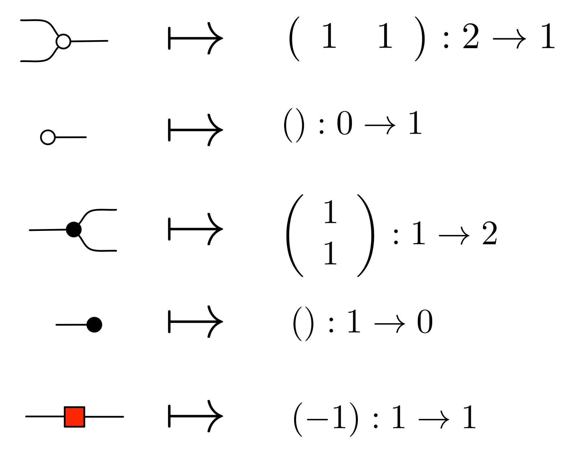
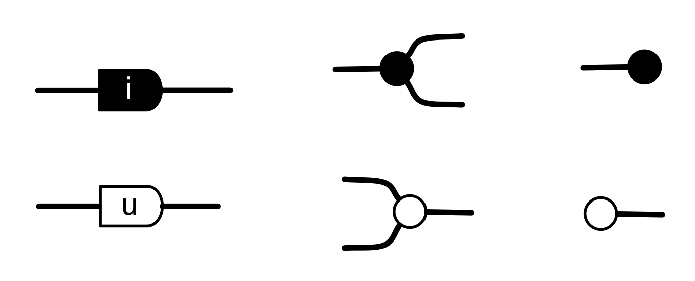
The cheat sheet for the diagrammatic system H  that includes the antipode is repeated below for easy reference.

cheat

We have already showed that H allows us to extend the syntactic sugar for natural numbers to a sugar for all the integers. We have also verified that the integer sugar obeys the usual algebraic laws of integer arithmetic. In particular, we proved that

minusonesquared

using the equations of H and diagrammatic reasoning: this is just -1 ⋅ -1 = 1, expressed with diagrams.


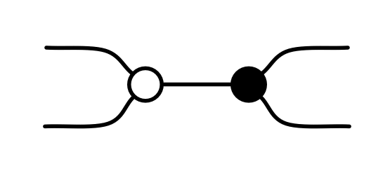
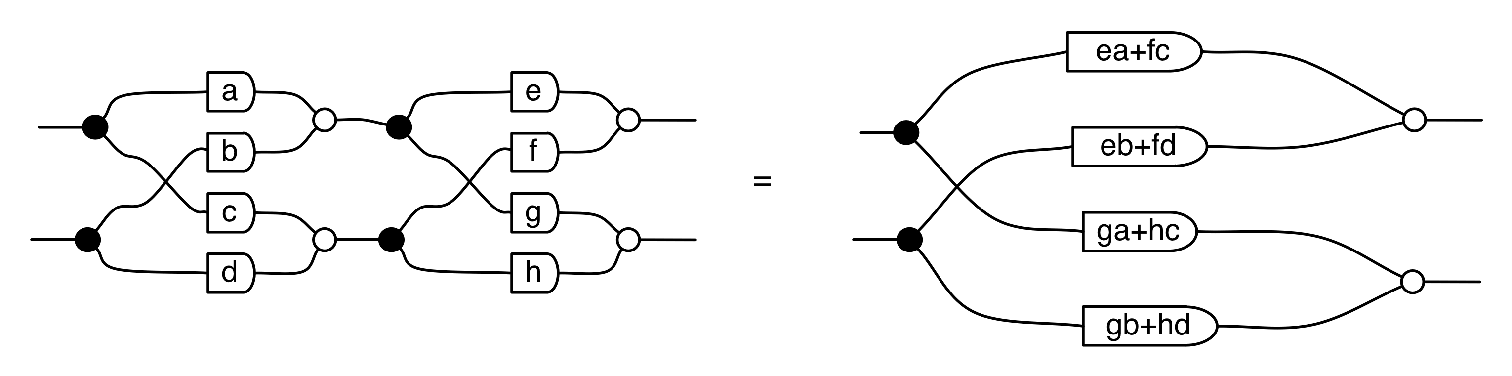
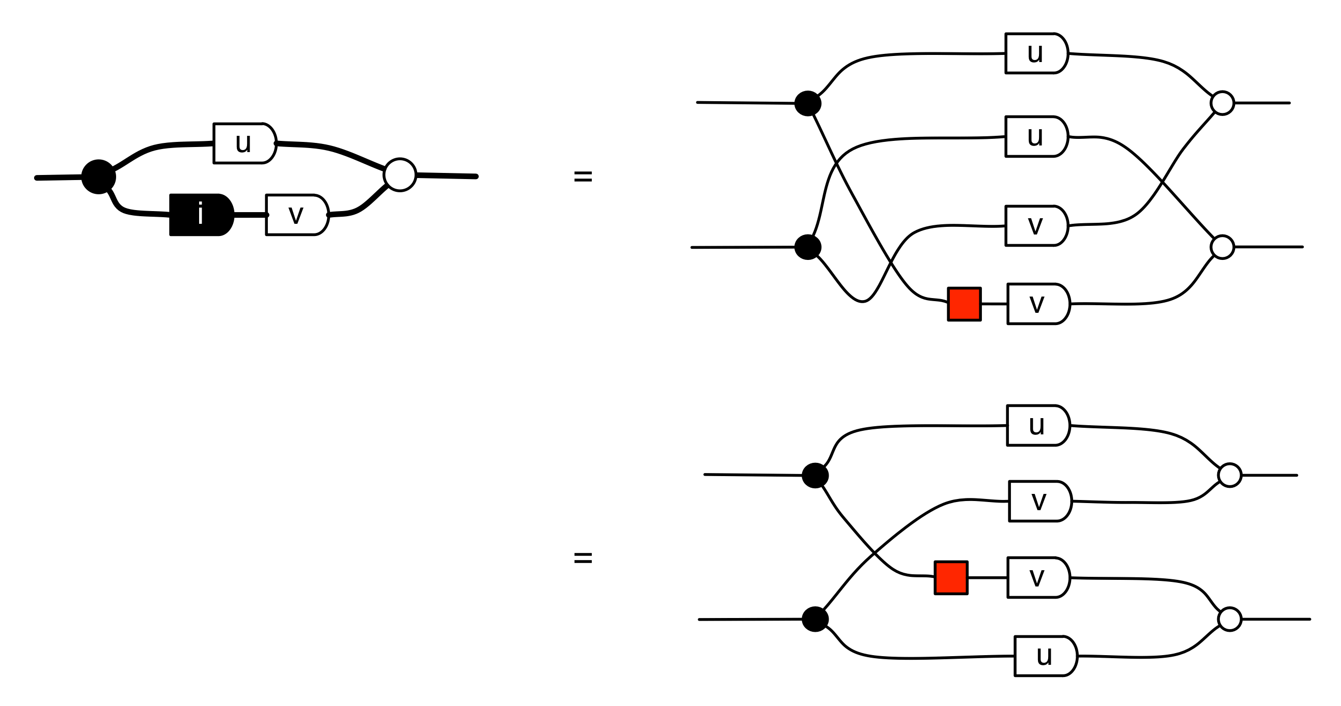
Let’s start with an example. The diagram below has two dangling wires on both sides.
iAs such, it ought to denote some 2×2 matrix, and to get the entry in the ith row and jth column we need to look at the paths from the jth dangling point on the left to the ith dangling point on the right.

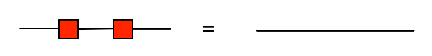
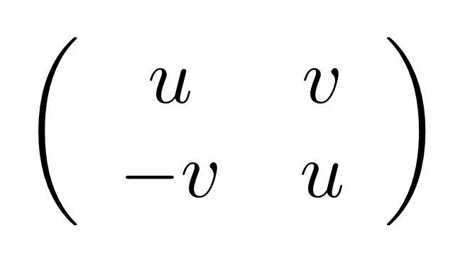
Before the antipode entered the frame, it sufficed to count the number of paths; the current situation is a little bit more complicated because there are positive paths—those on which the antipode appears an even number of times—and negative paths, those with an odd number. To get the relevant integer entry, we need to take away the negative paths from the positive paths. So, in the very simple example above, we have exactly one positive path from the first point on the left to the second point on the right, and one negative path from the second point on the left to the first on the right. The corresponding matrix is therefore:

imat

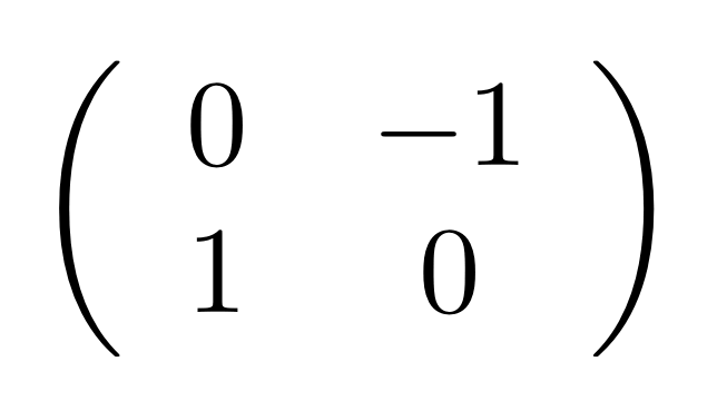
Actually, I didn’t choose this matrix at random: it allows us to consider the complex integers (sometimes called the Gaussian integers) and their algebra in a graphical way. We will come back to this after tackling the main topic for today.


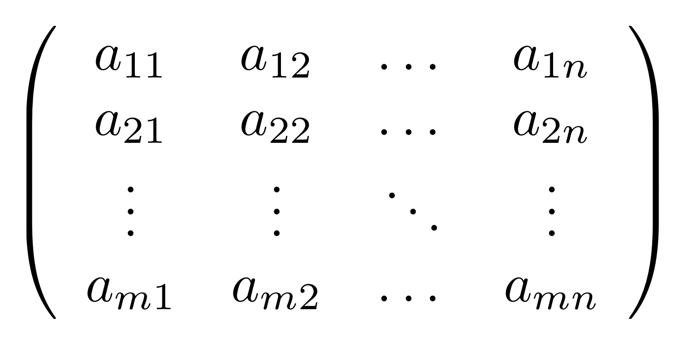
We want to prove that H is isomorphic to the PROP MatZ of matrices with integer entries. The letter Z is often used to mean the integers, from the German word Zahl meaning number; this notation was apparently first used by Bourbaki.

MatZ is similar to the PROP Mat that we discussed in Episodes 12 and 13: the arrows from m to n are n×m matrices, and just like before composition is matrix multiplication. The monoidal product is again direct sum of matrices.

The proof H ≅ Mat(the symbol  is notation for isomorphic to) is similar, and not much more difficult than the proof, outlined in Episodes 15 and 16, of ≅ MatLet’s go through the details.

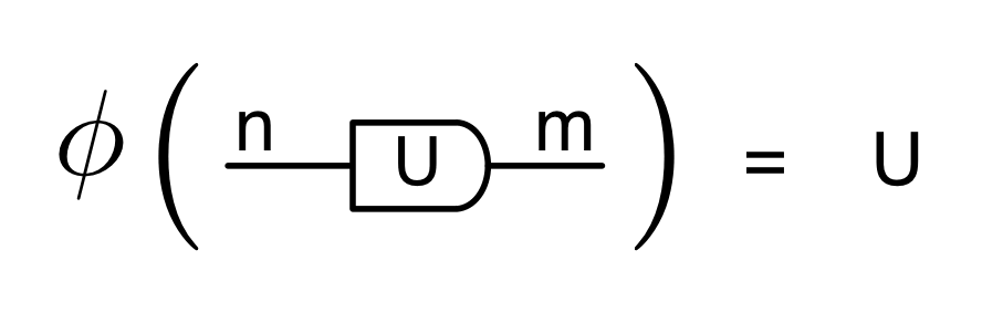
First we define a homomorphism of PROPs from H to MatZ. Let’s call it φ, the Greek letter phi. Since both H and MatZ are PROPs, and H is a free PROP built from generators and equations, it is enough to say where φ sends all the generators, and then check that the equations of H hold in MatZ.

It turns out that φ works the same way as θ for all of the old generators. The new part is saying where the antipode goes, and not surprisingly, it is taken to the 1×1 matrix (-1). Like so:

phi

For φ to be well-defined, we need to check that all the equations of  H also hold in MatZ. Fortunately, most of that work was already done for θ, we only really need to check the new equations that involve the antipode. Let’s check the most interesting of these, (A1); we need to calculate whether the following is true:

phia1

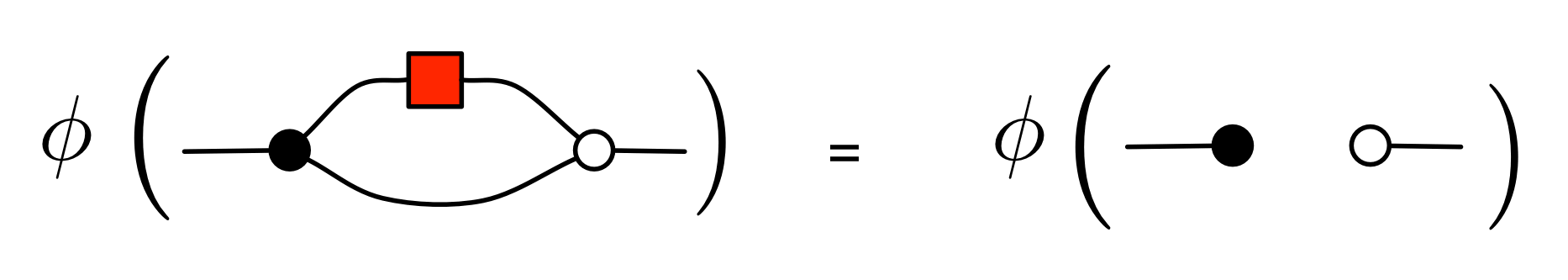
This amounts to checking if

phia1t

and it does, indeed, work. The other equations, (A2) through to (A5) are similarly easy computations and we will skip them; but feel free to check!


So we have a homomorphism φ: H → MatZ. To show that it is an isomorphism, we will show that it is full and faithful. Fullness—the fact that every matrix has a diagram that maps to it via φ—is the the easy part.

First, we need to check that the sugar that we defined in the last episode works with φ as expected, which is confirmed by the following simple calculation:

negsugarv

Any matrix with integers as entries can now be constructed following the procedure described in Episode 15. We will skip the details, as it is all pretty straightforward! The upshot of the construction is that we can extend the sugar for natural number matrices to a sugar for integer matrices: given an m×n integer matrix U we obtain a sugar

matrixsugar

such that

fullness

This establishes that φ is full.


So what about faithfulness, the property that says that whenever two diagrams map to the same matrix then they must already be equal as diagrams?

The trick is to get our diagrams into the form where the

copying comes first, then the antipodes, then the adding  (★)

One way of doing this is to use the theory of distributive laws. Eventually we will go through all of this properly, but for now I will just give you a high-level executive overview. The main insight is that we have three different distributive laws, the first involving the adding and the copying (B1)-(B4), the second the antipode and copying (A2)-(A3), and the third the antipode and adding (A4)-(A5).

The three distributive laws, are compatible with each other in a sense identified by Eugenia Cheng in her paper Iterated distributive laws. The fact that the distributive laws play together well in this way gives us the factorisation (★) that we want. We will discuss Cheng’s results in more detail in a later episode. Incidentally, she has recently written a book about category theory and recipes; I wonder if she knows about Crema di Mascarpone!


We could also try a rewriting argument, taking for granted that the rewriting system described in Episode 16 terminates.  Adding the following rules

rew

it seems that the expanded system ought to terminate also, although I have not yet got around to proving it. These termination proofs are always really messy for a rewriting amateur like me; I would love to hear from an expert about how to do these kinds of proofs in a nice way.


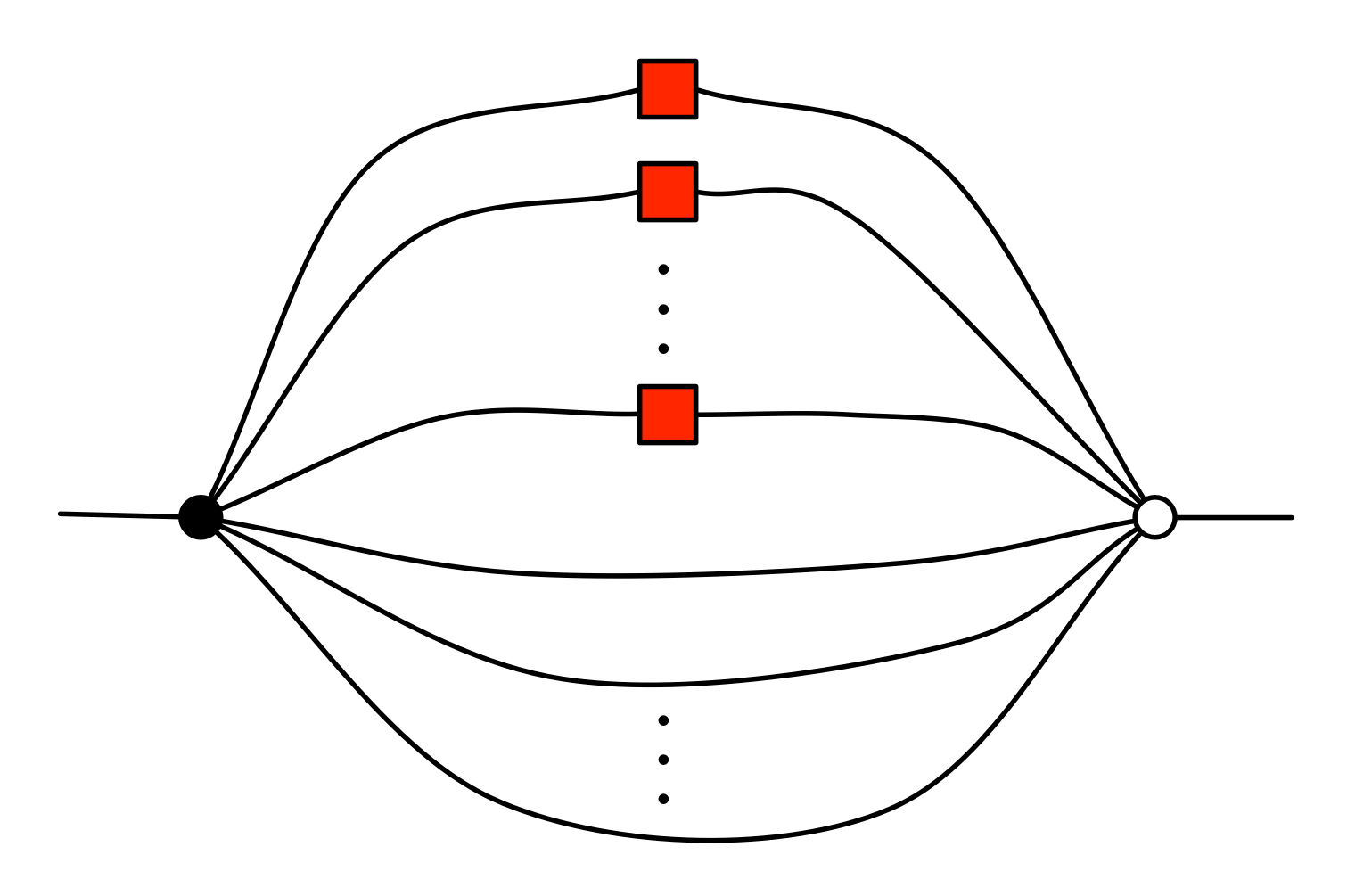
Once we know that every diagram can be put in the form (★), the proof of faithfulness is fairly straightforward. We start with those diagrams that have one dangling wire on each side. Every such diagram in the form  (★)  is either the sugar for 0 (a single discard followed by a single zero) or it can be rearranged into the form:

1-1

for some natural number k of wires with one antipode and some natural number l of wires with no antipode. This is because we can always get rid of redundant discards and zeros with (Counit) and (Unit), cancel out multiple antipodes in series using (†), then rearrange, and eat up any annoying permutations with the iterated copy and add sugars.

Once our diagram is in this form we can desugar and repeatedly use (A1), each time destroying one pair of antipode wire and no-antipode wire. Either we end up with no antipodes left, in which case the diagram is equal to a non-negative sugar, or we end up with some number of antipode wires. In the latter case, we can use (A2) to pull out the antipode to the left, obtaining the sugar for a negative integer. We have thus shown that faithfulness holds for the (1,1) case, since every such diagram is equal to some integer sugar.

The general case, where diagrams can have any number of wires on the left and right, comes down to transforming the diagram in matrix form, as explained in Episode 16. This step completes the proof that φ is faithful, and since we already know it is full, it is an isomorphism.


So far we have been identifying “numbers” with diagrams of a particular kind; those with one dangling wire on each end. In B this gave us the natural numbers, and in H it gives us the integers. But, as argued in Episode 17, there’s nothing particularly special about (1, 1) diagrams; well, maybe apart from the fact that both in B and H composition for (1,1) diagrams turns out to be commutative. Our obsession with the (1, 1) case is due to history—the traditional way of doing matrix algebra means the concept of ‘number” comes first, then the concept of “matrix”.

The complex numbers are a nice example where it makes sense to consider “numbers” as something different than (1,1) diagrams  A complex number can be written as an expression r + si where rs are numbers and i is a formal entity that behaves like a number, but with the mysterious property i= -1. The numbers and s are sometimes called, respectively, the real component and imaginary components. What is important for us is that to describe a complex number, it suffices to keep track of two ordinary numbers.  Our intuition is that wires carry numbers, so it makes sense to carry a complex number with two wires, the first for the real piece, the second for the imaginary piece.

complexintuition

Now if we multiply a complex number r + si by i, we get (r + si)i = ri + sii = -s + ri. So what was the real component becomes the imaginary component, and the negative of what was the imaginary component becomes the real component. We have a diagram for that, and we have already seen it in this episode:

iint

It thus makes sense to call this diagram i:

idef

Now if we multiply r + si by an integer u, we get (r+si)u=ru + sui. So both the components are multiplied by u. We also have a diagram for that:

scalarsugar2

where on the right hand side we used the sugar for integers from the last episode.

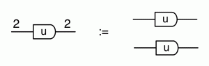
For the rest of this section, to stop the proliferation of the digit 2 that clutters the diagrams, we will just draw the 2 wire using a thicker line, like so:

thick

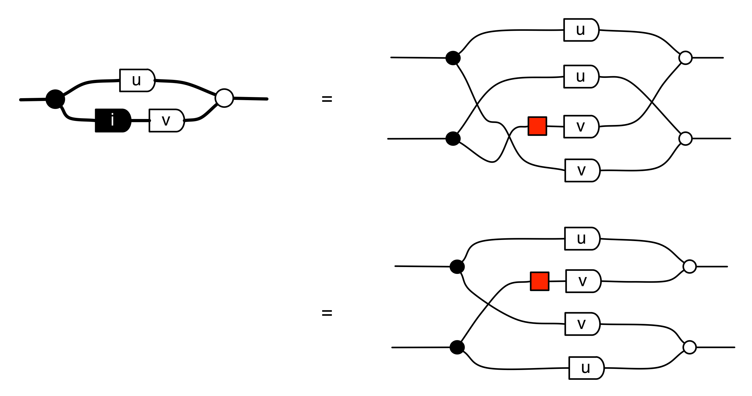
Now we can do some calculations. First if we compose the diagram for i with itself we get:

isquared

We can also show that i commutes with integers:
icommutes

Following the general pattern of this blog,  we can ask what kinds of diagrams one can construct using the following gadgets.
componentsUsing our standard box of tricks for reasoning about diagrams, it is not difficult to show that the diagrams with one thick wire on each side will, in general, be of the form:

gaussint

Composing two such entities gives us

gaussianmult

which is of course what you’d get if you multiplied out two complex integers (those complex numbers u+vi where u and v are integers). In general, the diagrams that can be constructed from bricks (‡) are matrices with complex integer entries.

So what exactly is going on here? Let’s take a look under the hood.

hood

The result is in matrix form, and corresponds to the 2×2 matrix:

mat

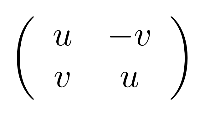
and this is known as one way of representing complex numbers using matrices.

There is one more interesting thing to say here. Let’s take a look at the bizarro of i.

bizarro

So the bizarro of i is -i. It follows that the bizarro of a general diagram constructed in the system (‡) corresponds to the operation known as conjugate transpose in complex matrix algebra.

If you know about quaternions, they can be considered in a similar way. Of course, we are constrained to integer coefficients for now. Not for long ☺.


I will give a 3 hour tutorial about graphical linear algebra at QPL ’15 in two chunks on Monday and Tuesday of next week. I’m desperately trying to get the slides done on time. Running this blog has been helpful in that it forced me to develop material, but unfortunately what we have covered so far will only be enough for around the first 30 mins; I should have started this blog back in January!

Continue reading with Episode 20 – Causality, Feedback and Relations.

Advertisement

16. Trust the Homomorphism, for it is Fully Faithful

Last time we proved that θ—the homomorphism that takes diagrams to matrices—is full. This means, roughly speaking, that for any matrix there is at least one corresponding diagram. Moreover, starting with an arbitrary matrix, we actually gave a recipe to construct a diagram that does the job. This provides us with a useful syntactic sugar, since any m×n matrix of natural numbers can now be considered as a diagram with n dangling wires on the left and m on the right. The construction extended the sugar for natural numbers from Episode 9.

There is still one final, thorny issue regarding θ that we ought to be nervous about. What if there are more diagrams than matrices? Or, more precisely, can we identify two different diagrams that go, via θ, to the same matrix? Then θ would not be perfect for the same reasons that “serendipity” and “dog” should not translate to the same word in French.

This final fear is laid to rest today as we tackle faithfulness. Once we know that θ is both full and faithful (or “fully faithful”) we can finally conclude that θ is a perfect translation; an isomorphism of PROPs.


The proof that θ is faithful is a little bit tricky. Let’s start by reminding ourselves of what faithfulness means: whenever two diagrams D1 and D2 are different, then the matrices θD1 and θD2 must also be different:

D1 ≠ D2     implies     θD1 ≠ θD2       ①

This is logically equivalent to saying that, for any diagrams D1 and D2, if θD1 happens to be equal to θD2 then D1 and D2 must have been equal to begin with.

θD= θD2     implies     D= D2           ②

In spite of the logical equivalence of and , the formulation in is somewhat easier to turn into a proof.  So let’s focus on what is saying. Given a diagram D, θD is table of numbers that record the numbers of paths from each dangling point on the left to each dangling point on the right in D. Then, to prove , we need to find a way of showing that:

whenever two diagrams have the same numbers of paths then they are equal.

And we consider two diagrams equal exactly when we can find a diagrammatic proof of this fact, using a combination of diagrammatic reasoning and our ten equations, repeated below.

cheat

We will outline two different ways to prove faithfulness. They both concern the four equations (B1)-(B4) that tell us what happens when adding meets copying. As we will see, the two different techniques each have their strengths and weaknesses, and for that reason it’s useful to have both in our toolbox.


The story naturally begins with diagrams that have a very particular shape: all of the copying comes before all of the adding. Let’s be a bit more precise: we mean those diagrams in which we can find a point to draw a vertical separator, so that the following condition is satisfied: the only generators allowed to the left of the separator are the black ones (copy and discard); and to the right of it the white ones (add and zero). Here’s a picture:

factorisation

and here’s an example of a diagram in this form.

ex1

To the left of the separator we have two copy generators, and to the right we have two addition generators and a twist. The twist is allowed on either side of the separator: this is because in our discussion about PROPs we understood that the twist is not a generator, even if we do consider it a basic brick of our diagrammatic language. The twist, aka σ1,1, is a part of the permutation structure expected in any PROP. In particular, another way of positioning the separator is the following, where the twist is now to the left of the separator.

ex2

Here’s a simple non-example for comparison:  we cannot find a place to put in a separator, because the addition comes before the copying.

ex3

Moreover, because the addition generator connects directly to the copy generator, we cannot use any of our vanilla diagrammatic reasoning, such as sliding along wires. We could, however, use the (B1) equation in our system to replace this diagram with the previous one, which has the right shape.

Most of the work of proving faithfulness is showing that every diagram can be transformed using our equations and diagrammatic reasoning into one in which the copying and the adding can be separated. This is because such diagrams are almost matrices, as we will now see.


Here’s what we mean by this rather cryptic remark: using the syntactic sugar for copy and add from Episode 10 together with the syntactic sugar for natural numbers  from Episode 9, we can easily transform any such diagram into matrix form. Diagrams in matrix form look like this:

matrixform

It’s easy to see that the matrix that results from applying θ to the diagram above is none other than:

matrix

So the entries can be read directly off the diagram: we simply scan down the centre to fill out the matrix.


Let’s go through an example to see how this works: it is not difficult to generalise the procedure to any diagram where the copying comes before the adding. Consider the diagram below. It is of the right shape, because we can draw a separator that walls off the black structure from the white structure.
step1We start by cleaning  the diagram up a little bit. We can use (Unit) and (Counit) to make some redundant zeros and discards disappear, and use diagrammatic reasoning to move the ones that remain so that they are right next to the boundary and don’t cause any further problems. In our example, this means using (Counit) to get rid of the discard at the bottom left, and pulling in the zero over on the right. We end up with the diagram below.

step1a

Next we introduce the syntactic sugar for copying and adding that gets rid of chains of copies and adds. In our example this means the following:

step2

Next we clean up even more: we eat up any annoying permutations (like the one at the bottom right) with the sugars, and collect compatible paths—those with the same dangling points—using our natural number sugar.

step3

We could really stop here, but being the pedantic sticklers that we are, we can slide the numbers along, and add 1s and 0s to get the diagram looking exactly like the template.

step4

But why bother to go to all this trouble?

The reason is that once we have a diagram D in matrix form, the relationship with its matrix θD is extremely tight since we can read off each matrix entry just by scanning down the middle of the diagram. This close connection can be exploited to prove faithfulness: when D1 and D2 are in matrix form, and θD1 is the same matrix as θD2, they clearly must be equal as diagrams!

So, in general, the question of faithfulness boils down to the following:

Can we transform any diagram into matrix form?

And, since we have just argued that any matrix in which copying comes before adding can be put into matrix form, the central question to consider becomes even simpler:

Can we transform any diagram so that copying comes before adding?

By the way, we have been putting diagrams in matrix form already without realising it. In Episode 10, we showed how go from the diagram on the left below—which totally fails to be in matrix form since some add generators come before copy generators—to the diagram on the right, which is in matrix form. The procedure of putting a diagram in matrix form is thus closely connected with the concept of matrix multiplication.

matrixmultdiag


It’s time to discuss one of the ways that we can answer the question. Putting the copying before the adding means focussing on what happens when the two structures interact. That story is captured by our four equations.

addingcopying

When we first discussed them in Episode 8, I mentioned that these equations amount to something called a distributive law of PROPs.

We will not go through the details of what this means now, but the upshot is that any diagram D can be factorised (a more fancy way of saying “transformed into a form in which we can find a suitable point to put in a separator”) so that D = C ; A, where C is a diagram that uses only the copy and discard generators, and A only the add and zero generators. So the work comes down to showing that the rules (B1)-(B4) actually amount to a distributive law. Fortunately, Steve Lack considers this very example in Composing PROPs, it is Example 5.3 in that paper. The deeper story behind all this is actually both extremely interesting and enlightening, but it requires a little bit more category theory. We will come back to it eventually.

Overall, the strength of using this technique is that… we didn’t really have to do very much. For austere, beautiful mathematical reasons, the equations give us a distributive law and guarantee that that the factorisations we need always exist. But if you give me a diagram and tell me to find an actual factorisation then I don’t have very much to go on: I know it exists, but the distributive law does not tell me how to find it. Nevertheless, it is enough to prove faithfulness, so we should not complain too much.


The second way of showing that every diagram can be factorised relies on a technique called rewriting. The basic idea is that, instead of considering (B1)-(B4) as equations, we orient them and consider them as rules.

rewriting

Then, the strategy is to find left hand side of one of the rules in our diagram. This is called a match for that rule, and if we can find it, we replace it with the rule’s right hand side. Next, we keep repeating these two steps until we there are no more matches. The rules take care of all the possible ways that white structure can come before black structure, so if we cannot find any matches then we have essentially found the factorisation.

Sounds simple enough, but there are a few complications. Let’s go through an example to get a feel for what’s going on. Our starting diagram is drawn below, and already we have found a match for one of the rules; it’s the area highlighted within the red rectangle.

rew1

So we replace the match with the right hand side of the rule, obtaining the diagram below.

rew2

The red box in the second diagram is highlighting another match, which we can then replace with a right hand side of the relevant rule. Let’s keep repeating this procedure to see where we end up.

rew3

rew4

rew5

rew6

Now we seem to be almost finished, but there’s still an add connected to a discard, highlighted in the last diagram above. We do have a rule for that, but the match is complicated by the fact that there is a twist in the middle. So, if we were going to implement this in software, we’d have to make sure that our algorithm for finding matches takes these kinds of situations into account. And after this final step the diagram becomes

rew7

where there are no more bad connections. We can now simply use diagrammatic reasoning to pull all of the black structure to the left and the white structure to the right, obtaining a factorisation.

Another, more radical, way to deal with the issue of matches is to go back to the drawing board and change the way we think about diagrams.  We have been thinking of diagrams as magic Lego, built up of basic tiles that connect to other basic tiles. But we could start thinking of them as graphs with white nodes and black nodes. Then, the rewriting we have been discussing becomes a kind of graph rewriting.

This is the approach taken by Aleks Kissinger at Oxford, who has developed the Quantomatic software package for working with string diagrams. Aleks and his collaborators have developed a whole load of really cool new technology, and I hope to convince him to eventually write a few articles on this blog, explaining some of the latest developments!

There is one more issue to consider when dealing with rewriting: termination. Let’s look at the first step of our rewriting example again. In the first diagram, there is only one match. But by applying the rewrite rule, we ended up in a diagram with three different matches. It seems that we’ve cut of the head of the Hydra only for three heads to pop up again. If this kind of thing continues indefinitely, then as much as we rewrite, we will never finish.

This thing about rewriting systems in general, is that:

  1. they may look simple and intuitive
  2. but it is often surprisingly tough to prove that they terminate.

Fortunately, the rewriting system above does terminate. We will prove it eventually on this blog, but you’re welcome to try it yourself; it’s not so trivial!

There are several people studying rewriting theory on diagrams like ours. For example, Samuel Mimram at the École Polytechnique has recently been doing some very exciting work on  techniques that simplify the process of proving properties like termination.


Summing up: if we use the distributive law then we don’t have to work very hard but we don’t get a factorisation algorithm. If we use rewriting then we have an algorithm but we have to work quite hard to prove that it works. Such is life.


This episode concludes the work of showing that θ is an isomorphism. We have spent quite a bit of time discussing the mathematics of diagrams. This was all very useful because, after all the hard work, we now have a much firmer handle on how to work with them. But, as interesting as it is, the mathematics of diagrams is not really the main point of this blog, which is doing mathematics with diagrams. This is the subject of the next episode.

Continue reading with Episode 17 – Maths with Diagrams