27. Linear Relations

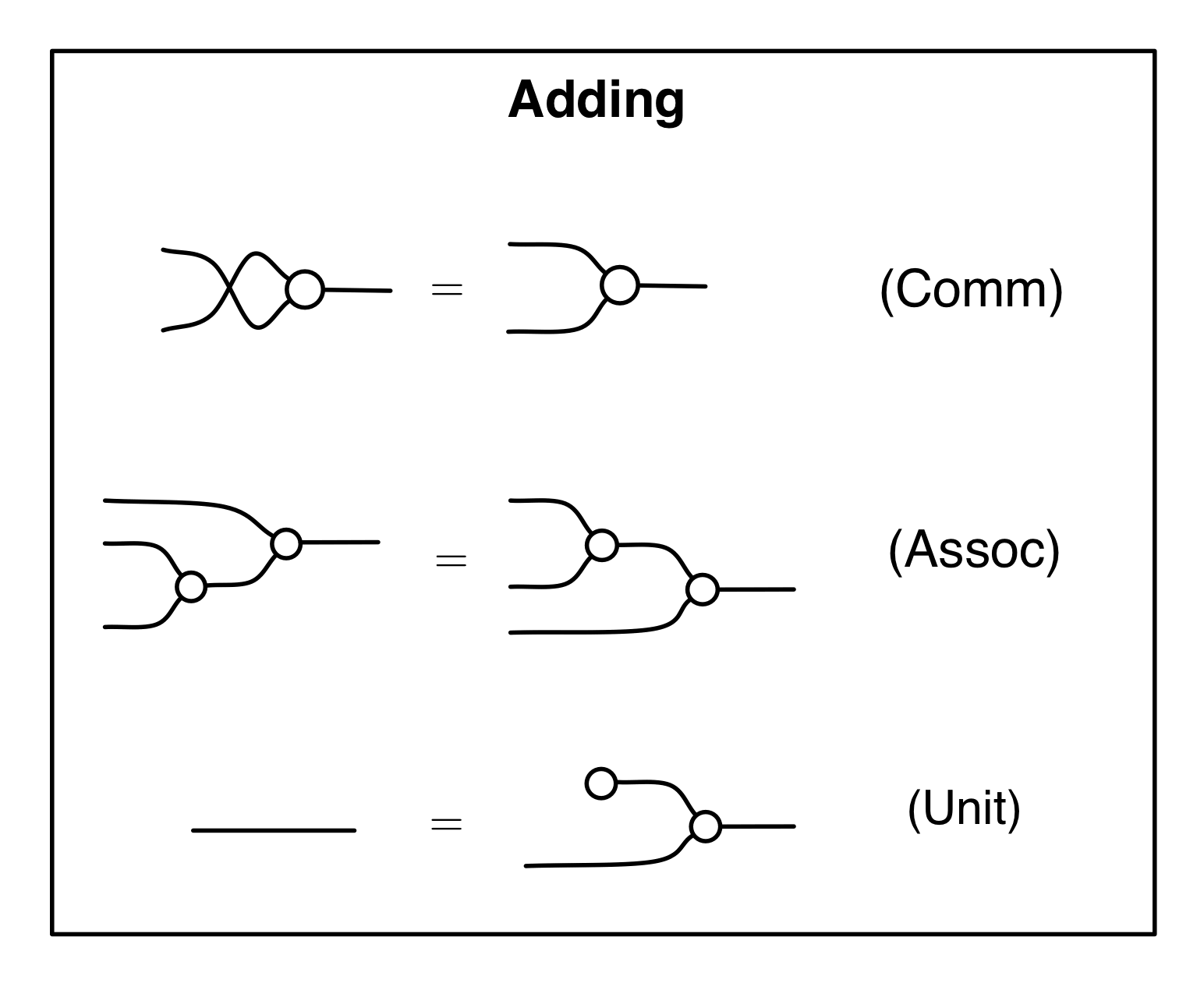
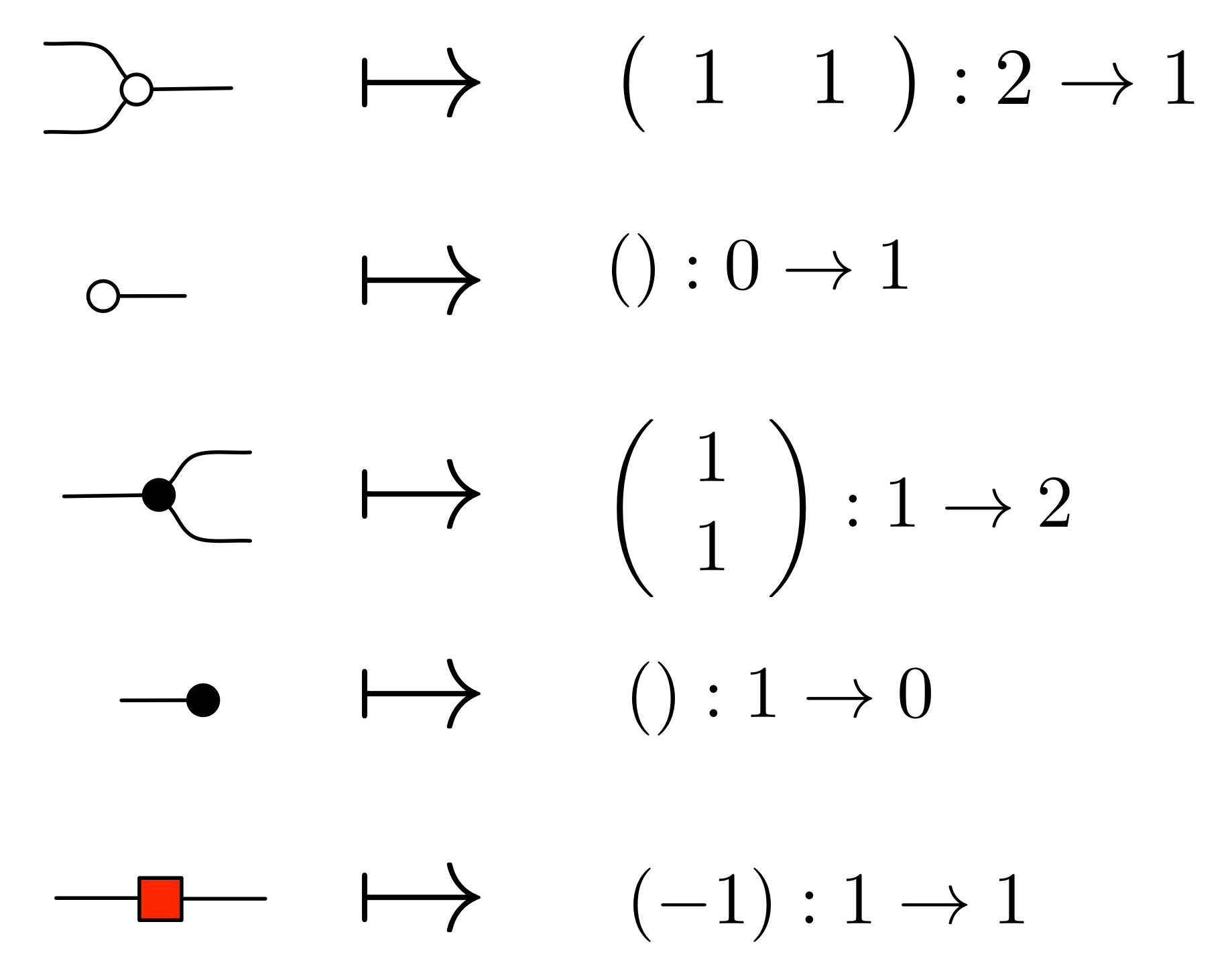
In the last two episodes we focussed on fairly simple diagrams in IH: those with just one dangling wire on each end. In this episode we expand our horizons and consider arbitrary diagrams. It’s time to return to linear algebra. We will also revisit division by zero from a different, but equivalent, point of view.

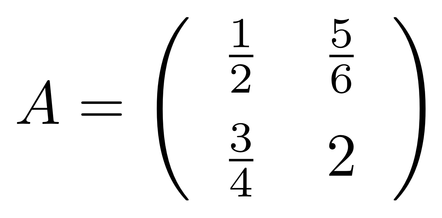
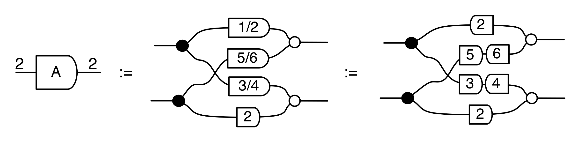
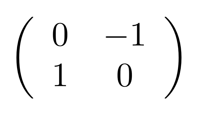
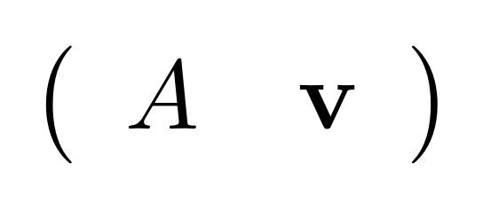
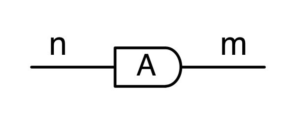
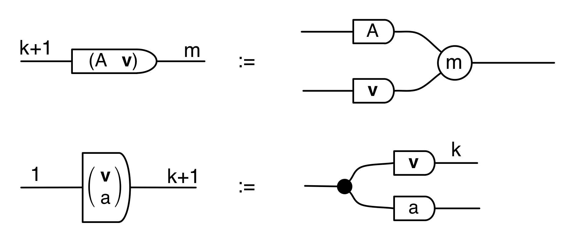
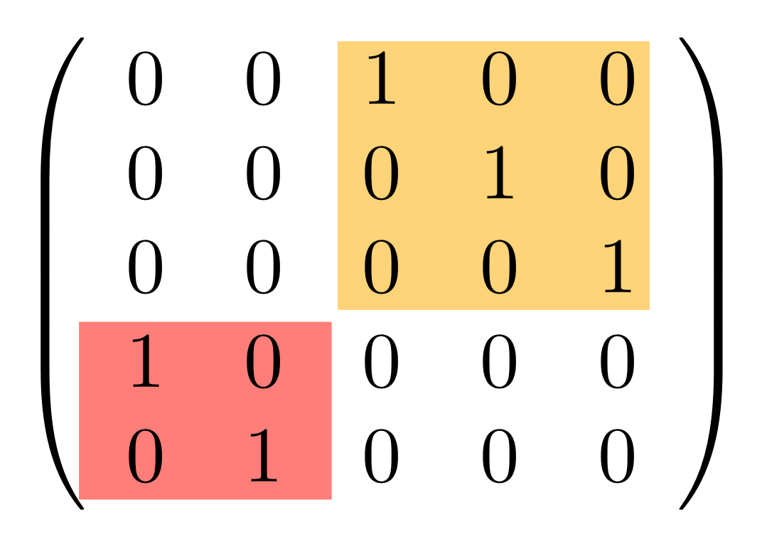
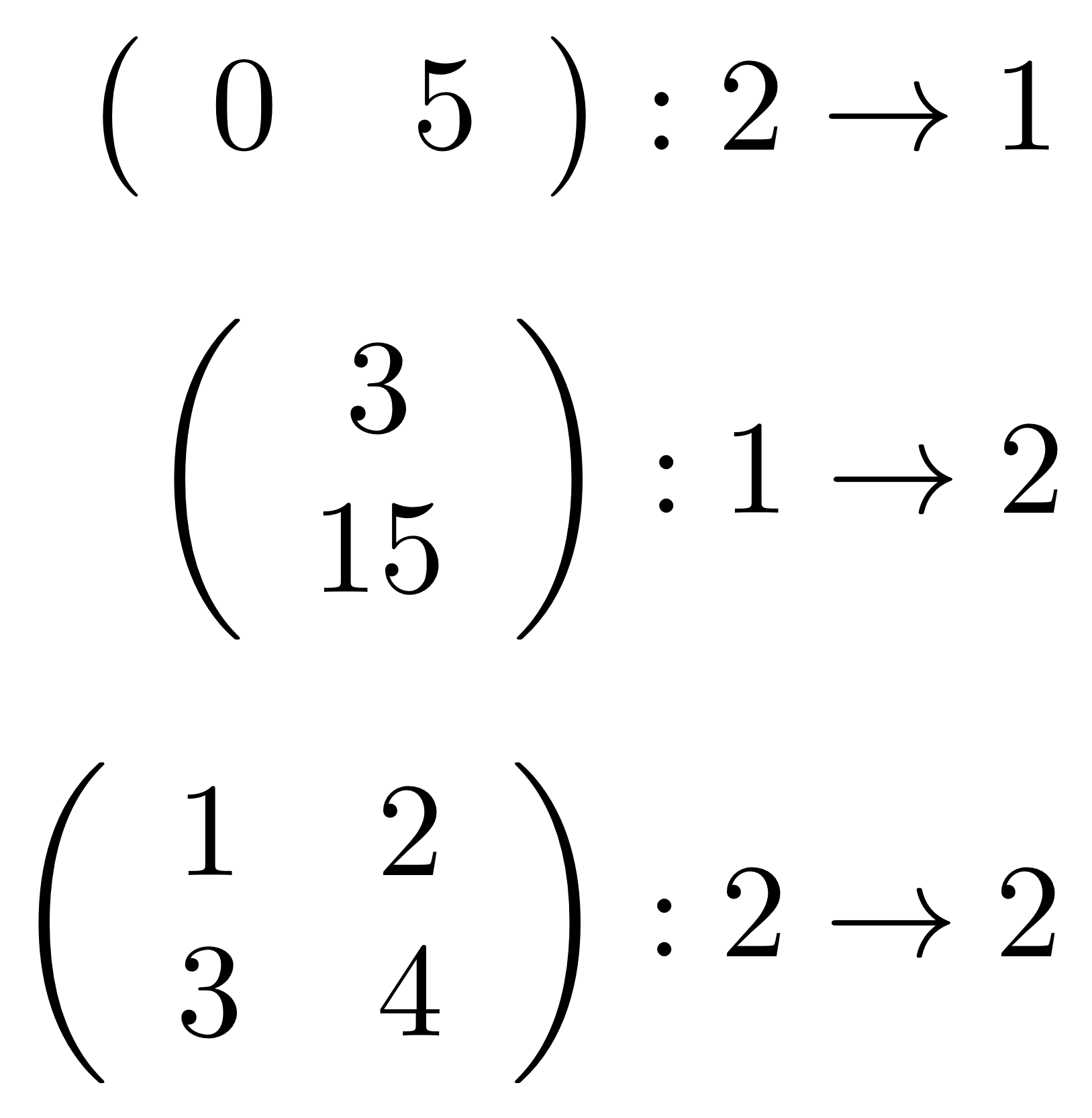
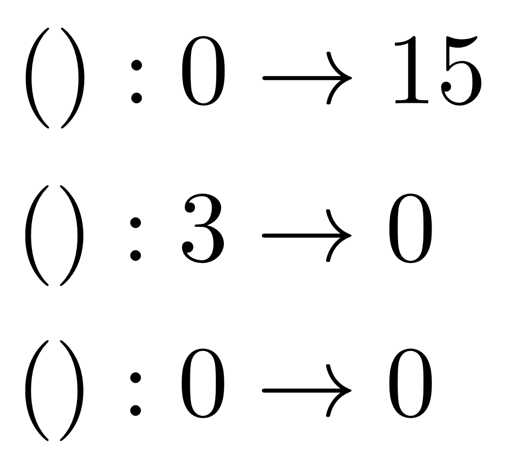
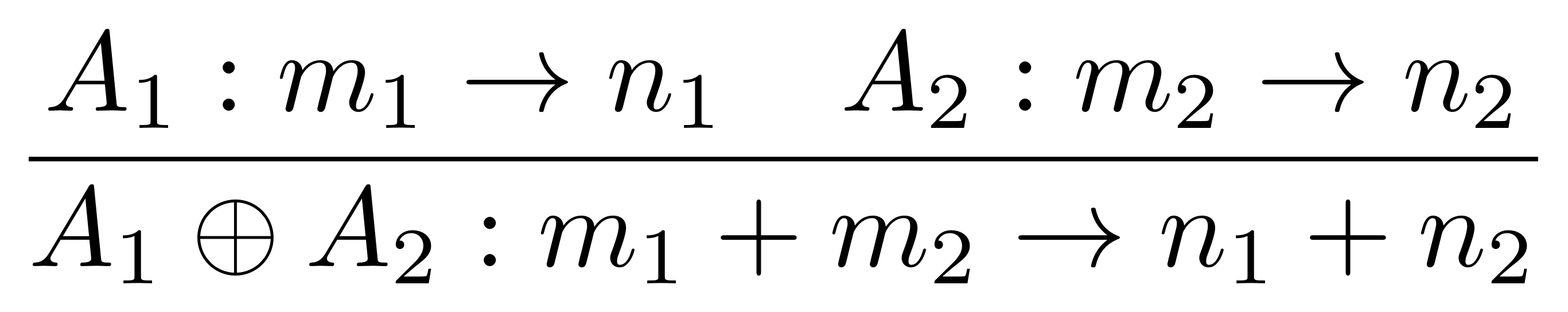
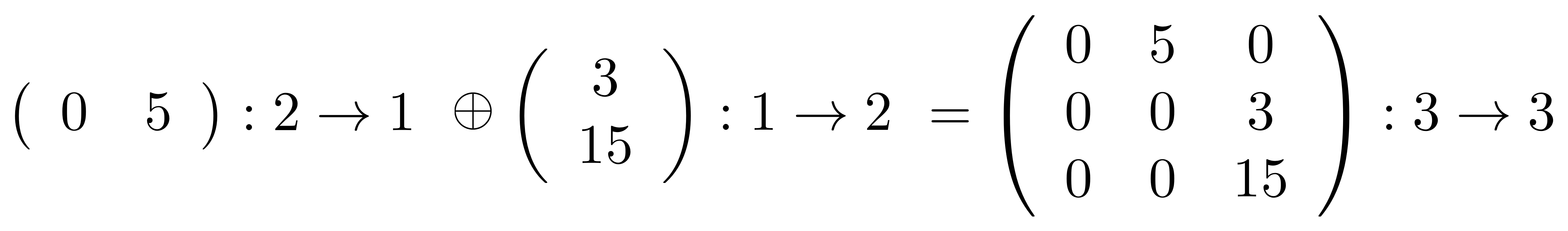
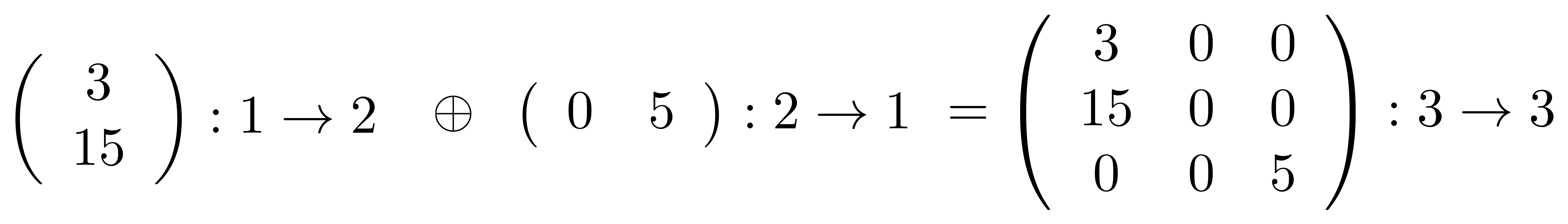
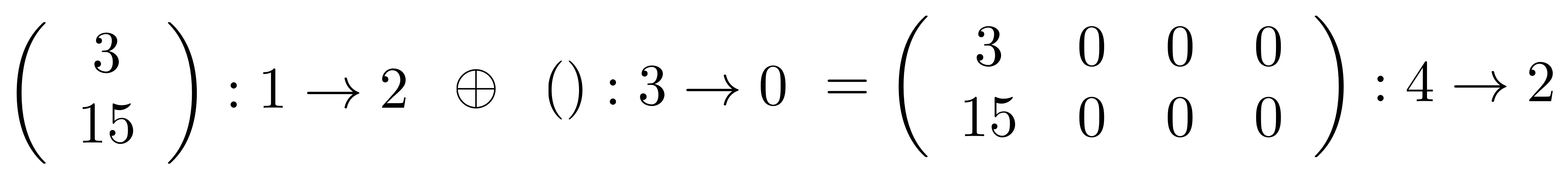
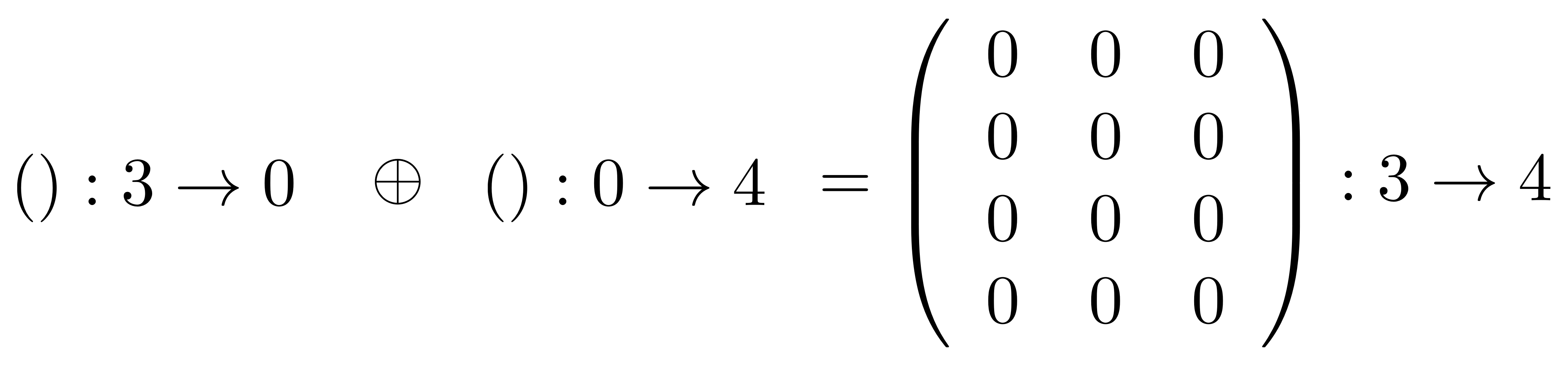
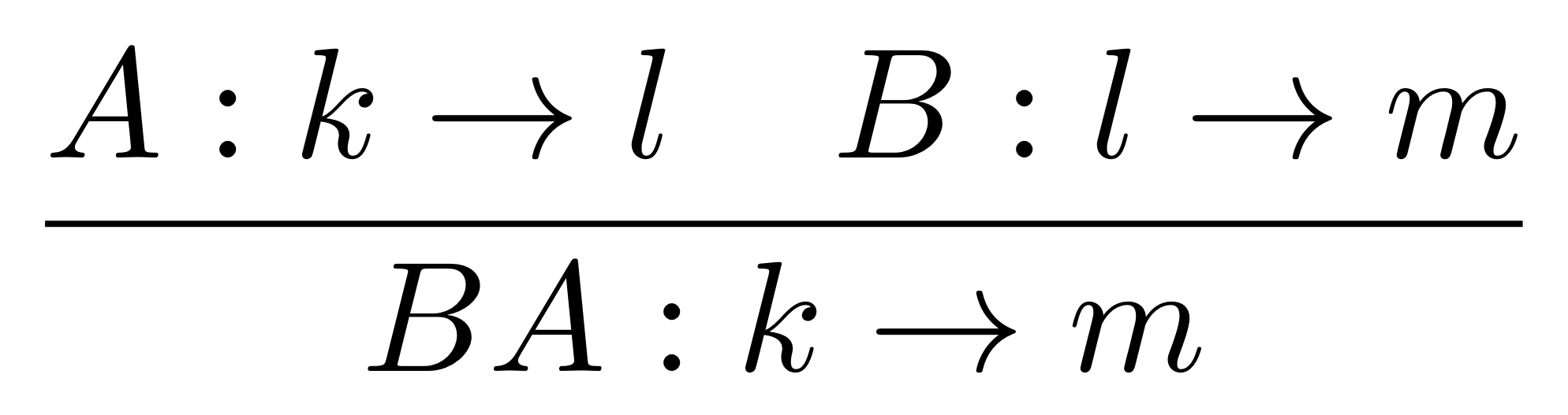
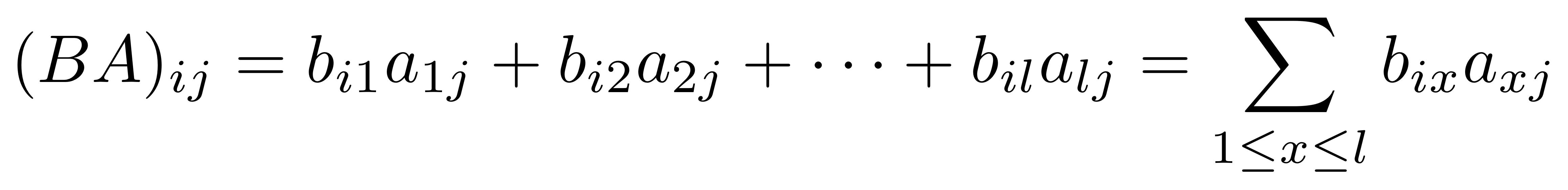
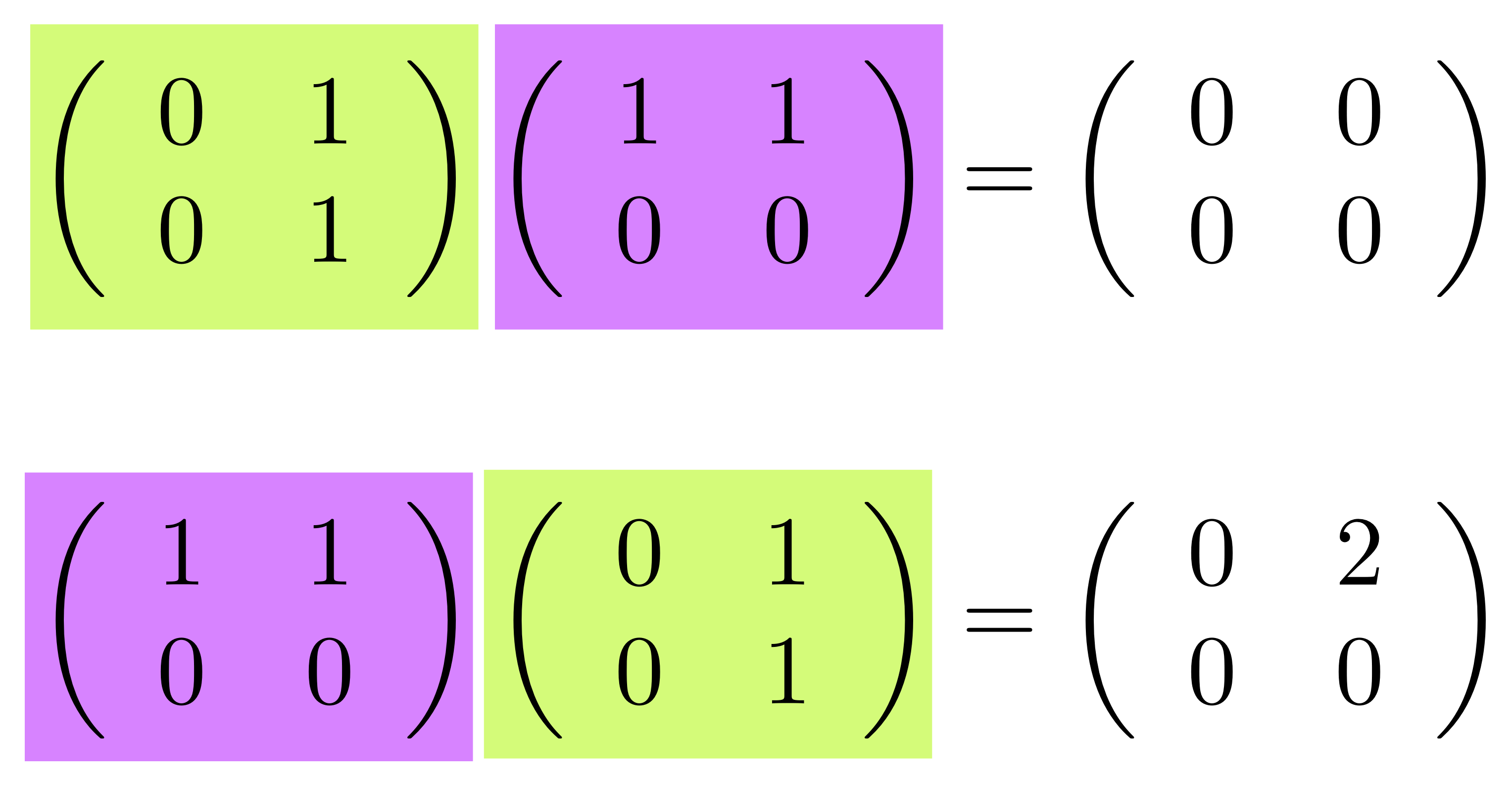
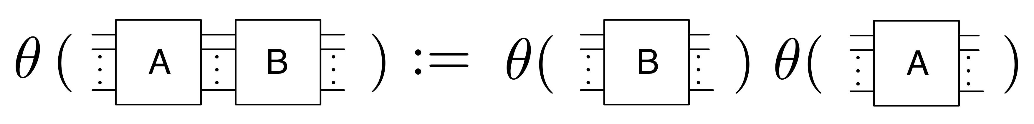
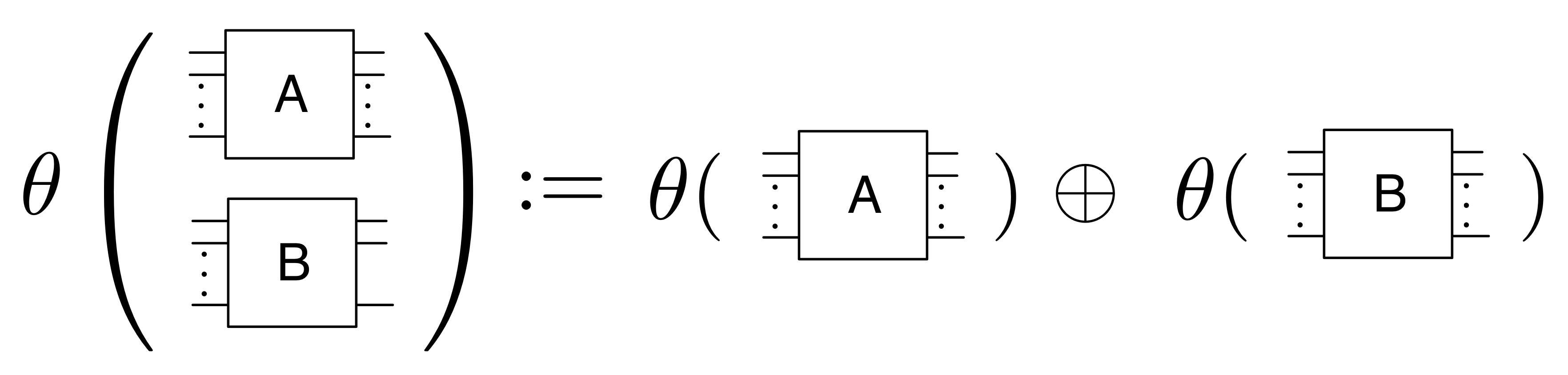
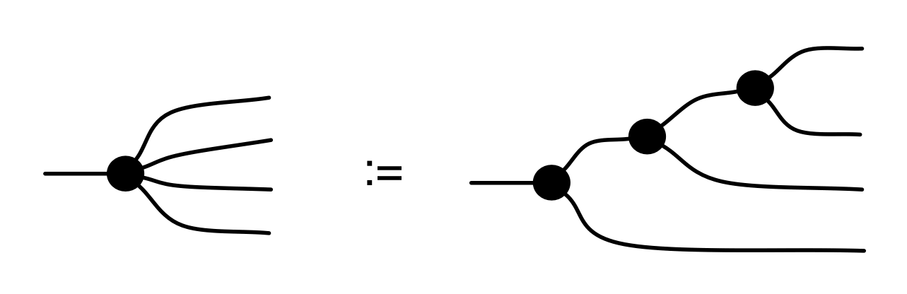
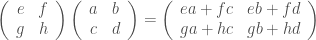
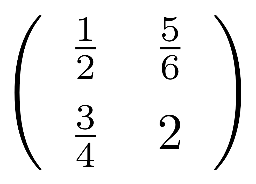
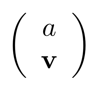
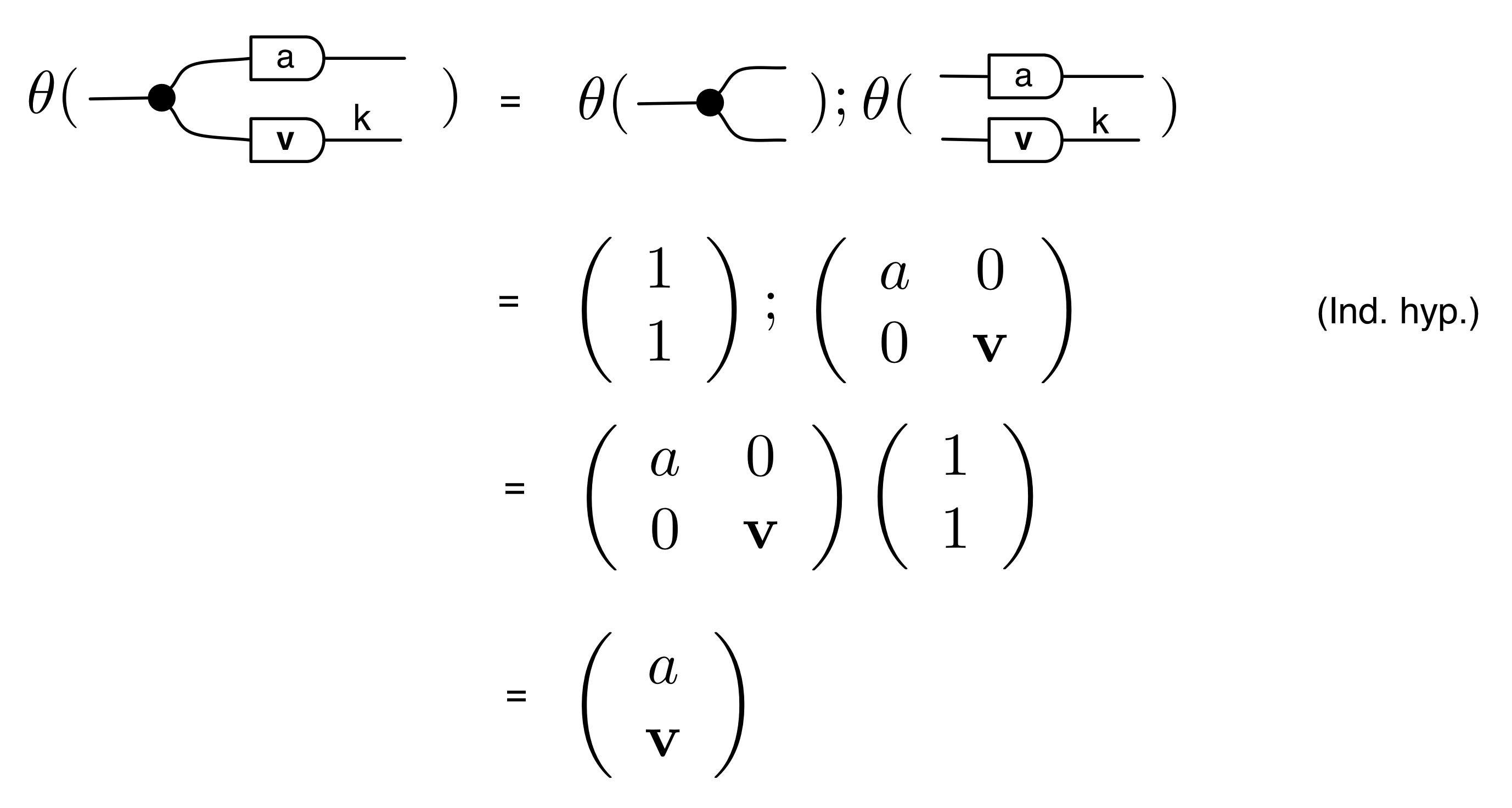
We’ve known since Episode 10 how to handle matrices diagrammatically, and since our expanded graphical language can handle fractions, we can put the two together and draw matrices of fractions. The algebra works as expected: if we restrict our attention to these matrices, composition is matrix multiplication, and the monoidal product of two matrices is their direct sum. Here’s a reminder of how to draw, say, the following matrix

$exmatfrac$

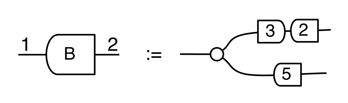
But we can do much stranger things. Since we have the mirror image operation † in our arsenal, we can consider matrices going backwards. We don’t have any traditional notation for this: how could you write a matrix that “goes backwards”? But here’s an example in the language of diagrams, if

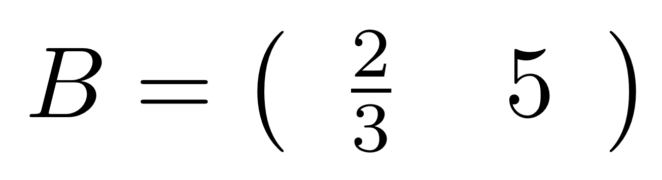
Then we have can draw the diagram for B going from right to left.

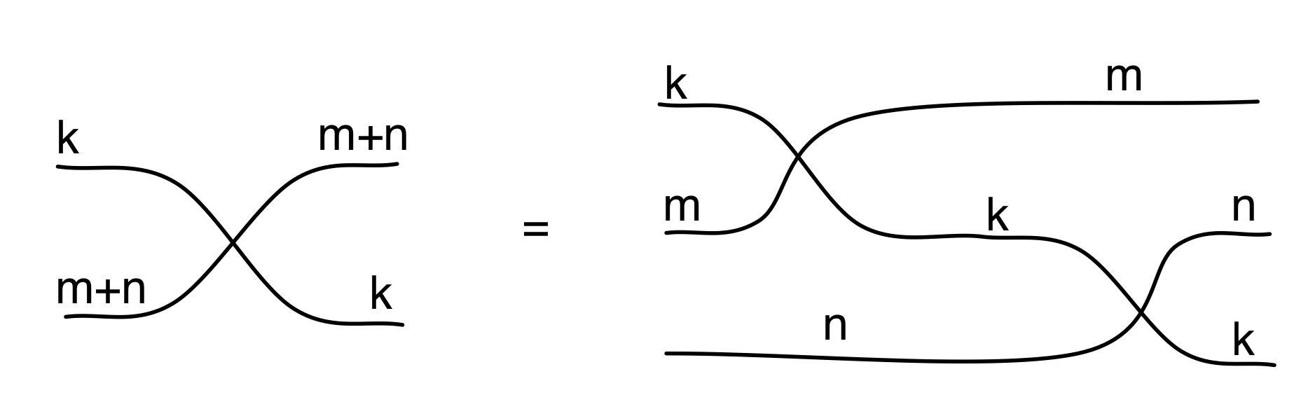
Matrices and backwards matrices are not the full story because diagrams can get more complicated. In general, diagrams from m to k will be quite strange beasts: imagine a zig-zag of matrices going back and forth. It’s as if we took our Lego and got confused about what are the studs and what are the holes. Everything goes.

Let’s clear up the mystery. We know that the sub theories B and H are isomorphic to, respectively, the props Mat of matrices of natural numbers and Mat_Zof integer matrices. Knowing this helped us to understand the diagrams in those theories, and what they were capable of expressing.

So, without further ado, it’s time to meet the linear algebraic prop LinRel that hides behind the equations of graphical linear algebra. Coincidently it’s my favourite category, so please forgive me if I sound a bit too much like a fanboy in the following. Before we start, we need some notation: in the following, the bold letter Q stands for the set of fractions, aka the rational numbers.

The arrows from m to n in LinRel are linear relations from Q^m to Qⁿ. Roughly speaking, LinRel is what happens when you combine matrices and relations. The result is truly delightful; it is much more than the sum of its parts. You will see what I mean.

Before I explain what linear relations are in more detail, let me first say that it’s a huge mystery that the concept of linear relation does not seem to be particularly standard or well-known: there is not even a wikipedia page at the time of writing this episode! Since there’s an informative wikipedia page about, say, Cletus from the Simpsons, this is a bit offensive. Maybe it’s because of a human preference for functional thinking, at the expense of relations? We discussed that a bit in Episode 20.

So what is a linear relation exactly?

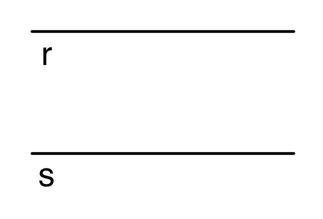
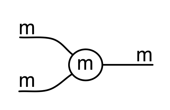
First, a linear relation of type Q^m ⇸ Qⁿ is a relation, so a subset of the cartesian product Q^m × Qⁿ. De-jargonifying, this means that it’s a collection of pairs, with each consisting of an m-tuple and an n-tuple of fractions. For example, the linear relation for the addition generator—which we have already discussed informally in Episode 22—is the relation of type Q²⇸ Q that consists of all pairs

where r and s are fractions. We have thus finally demystified what the enigmatic universe of numbers Num is: for now Num = Q, our numbers are fractions.

We still need to account for the word linear in linear relations. Said succinctly, to be linear, a relation R: Q^m ⇸ Qⁿ must be a linear subspace of Q^m × Qⁿ, considered as a Q vector space. If you don’t know what those words means, let me explain.

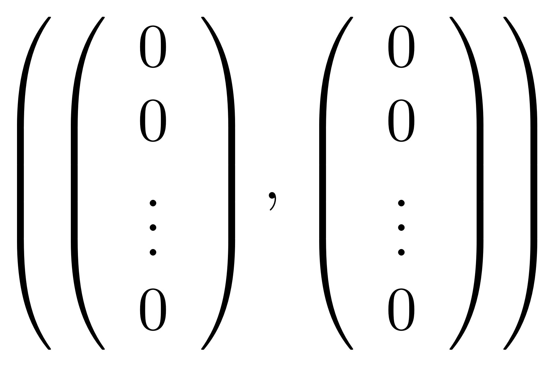
First, R must contain the pair of zero columns.

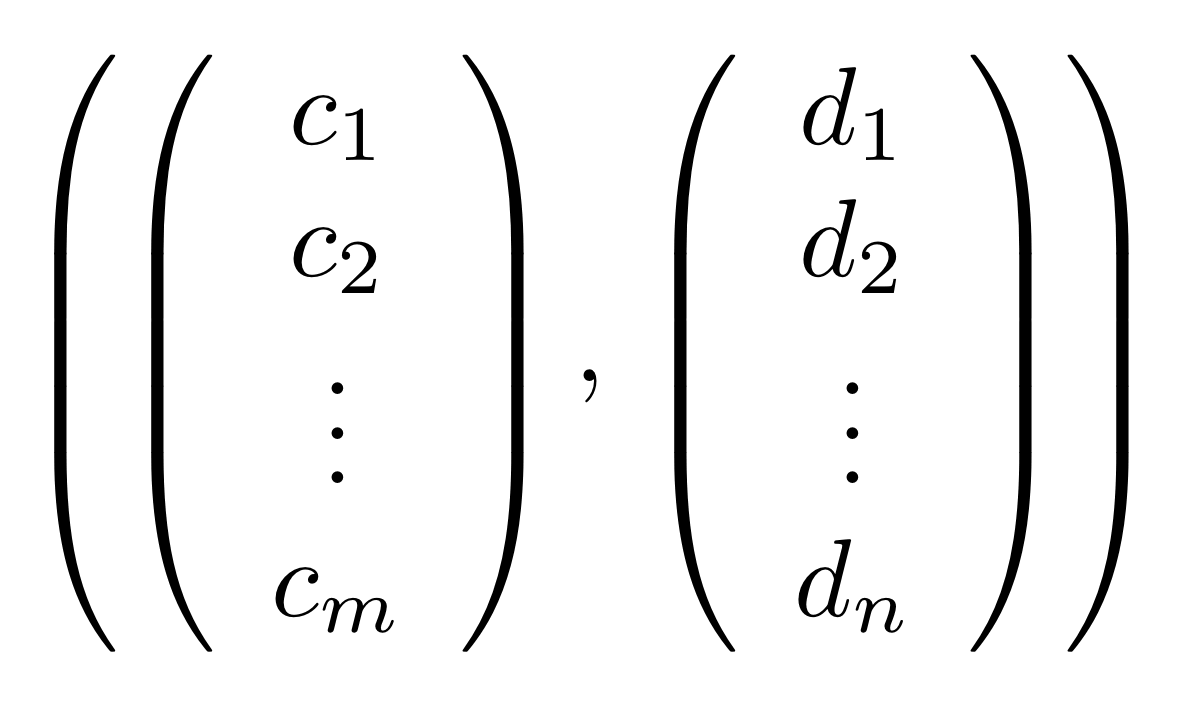
R must also satisfy two additional properties.The first is that it must be closed under pointwise addition. This scary sounding condition is actually very simple: if R contains pairs

and

then it also must contain the pair obtained by summing the individual numbers:

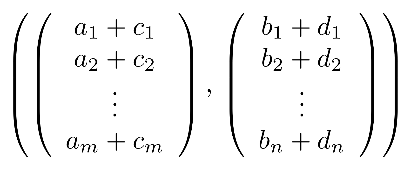It takes a lot of space to write all those columns, so let’s introduce a common notational shorthand: we will write a for the a-column (or column vector), b for the b-column and so forth. When we write a+c we mean that a and c are columns of the same size and a+c consists of a₁+c₁, a₂+c₂ and so on until a_m+c_m. So—using our new shorthand notation—for R to be closed under pointwise addition, whenever (a, b) and (c, d) are both in R then also

(a, c) + (b, d) := (a+c, b+d)

must be in R.

The second property of linear relations is that they must be closed under scalar multiplication. This means that whenever

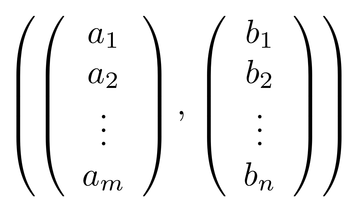
is in R then also

must be a member, where k is any fraction. We can also do say with the shorthand notation: given a vector a and fraction k, we will write ka for the vector with entries ka₁, ka₂, …, ka_m. So, being closed under scalar multiplication simply means that if a is in, then ka must also be in.

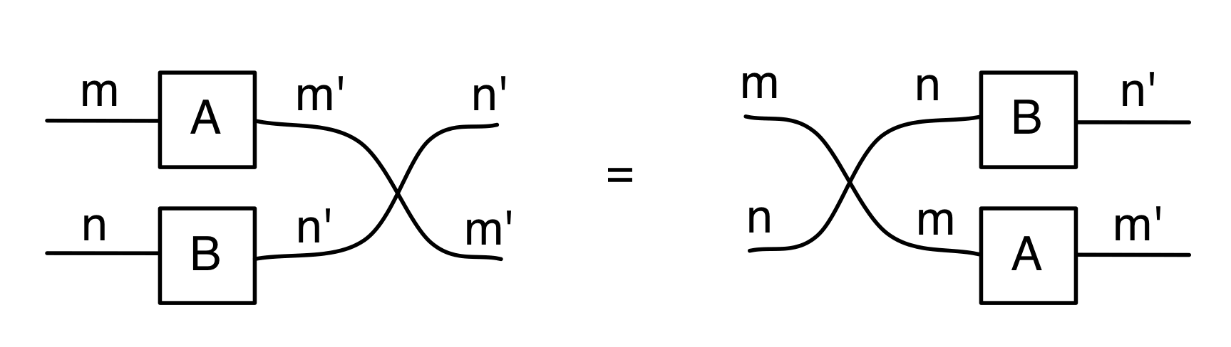
Composition in LinRel works just like it does in Rel, so composing R: Q^m ⇸ Qⁿ and S: Qⁿ ⇸ Q^p gives R;S : Q^m ⇸ Q^p with elements (x, z) precisely those for which we can find a y such that (x, y) is in R and (y, z) is in S.

I claim that LinRel is a prop. To be sure, we need to do some things that may not be immediately obvious:

verify that the identity relation is a linear relation,
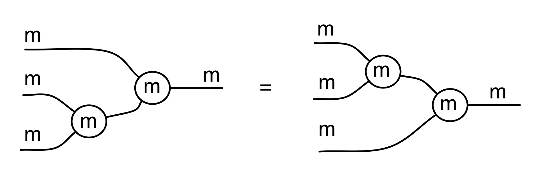
check that composing two linear relations results in a linear relation, and
say what the symmetries are and make sure that they work as expected.

The first one is easy, try it!

For point 2, we need to show that if R: Q^m ⇸ Qⁿ and S: Qⁿ ⇸ Q^p are linear relations then so is R;S.

Let’s prove closure under pointwise addition: suppose that (x₁, z₁) and (x₂, z₂) are in R;S. We need to show that (x₁+x₂, z₁+z₂) is also in R;S. Using the definition of relational composition, there exist y₁, y₂ such that (x₁, y₁) and (x₂, y₂) are both in R and (y₁, z₁) and (y₂, z₂) both in S. Since R and S are linear relations, they are both closed under pointwise addition, so we can conclude that (x1+x₂, y₁+y₂) is in R and (y₁+y₂, z₁+z₂) is in S. It thus follows that (x1+x₂, z₁+z₂) is indeed in R;S. I’ll leave you to check that it’s closed under scalar multiplication, the argument is very similar.

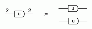
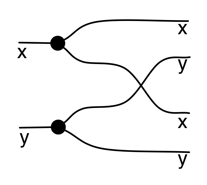
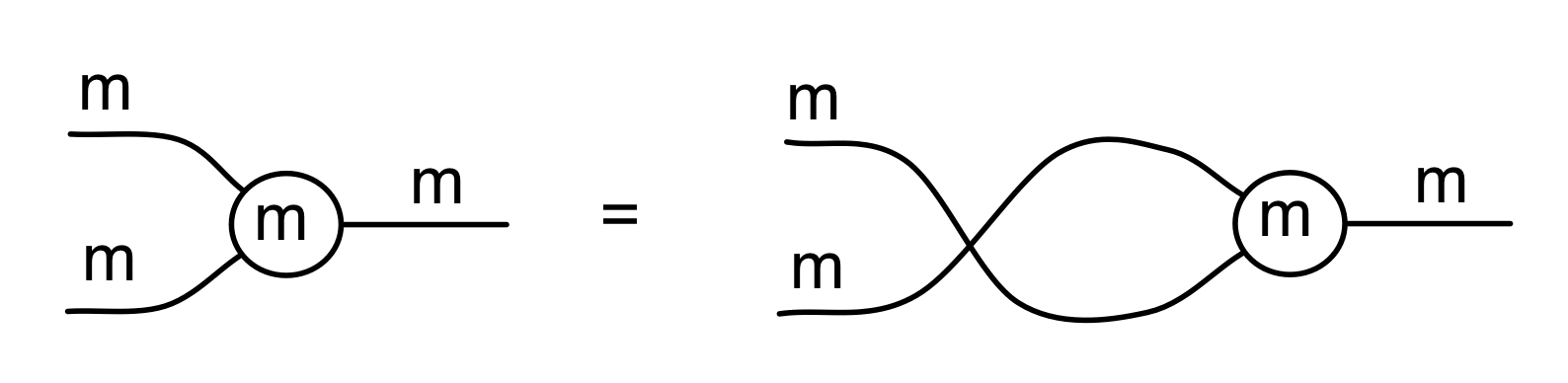
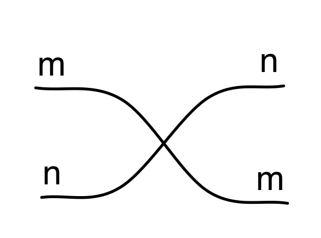
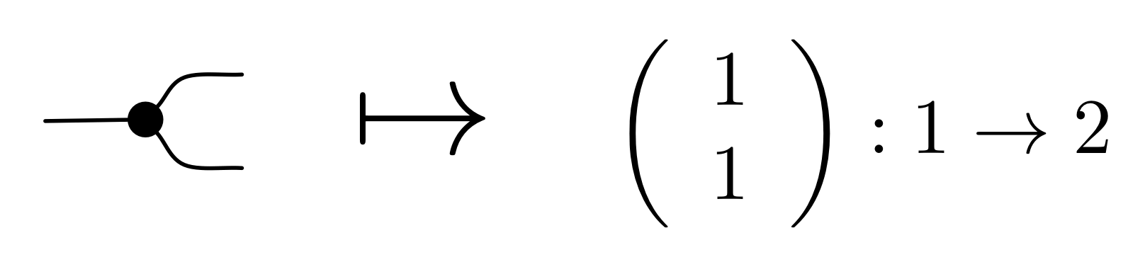
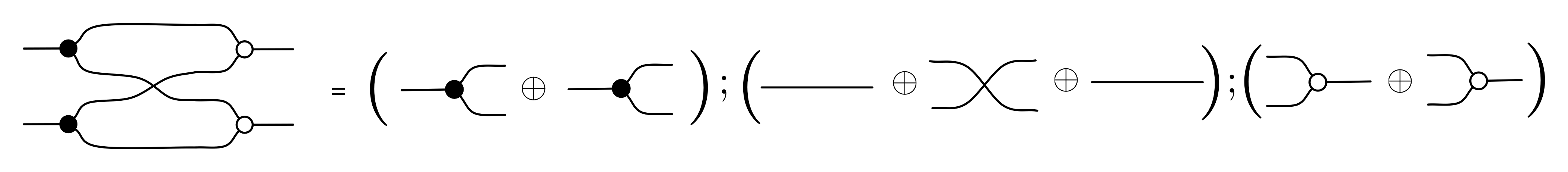
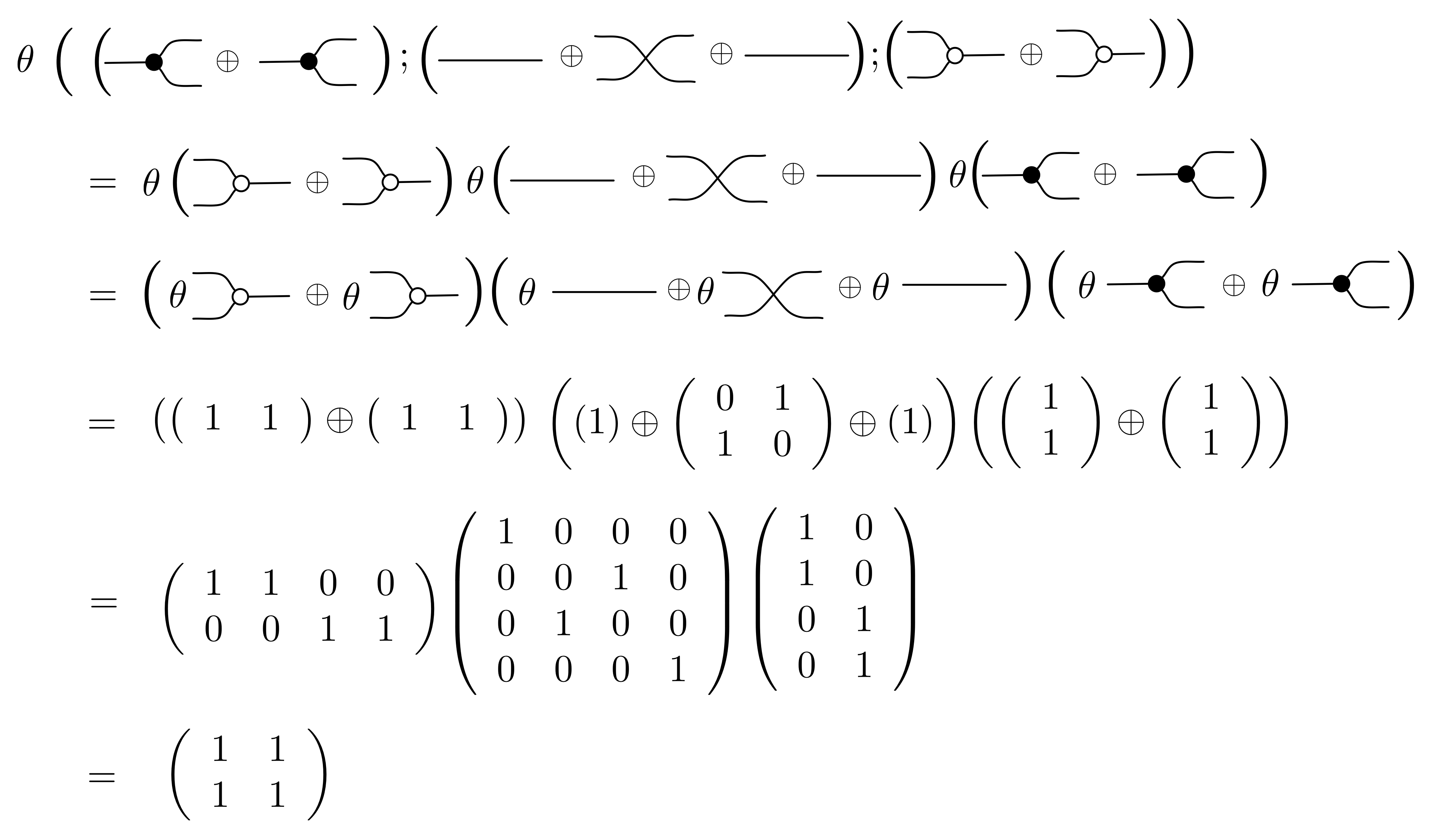
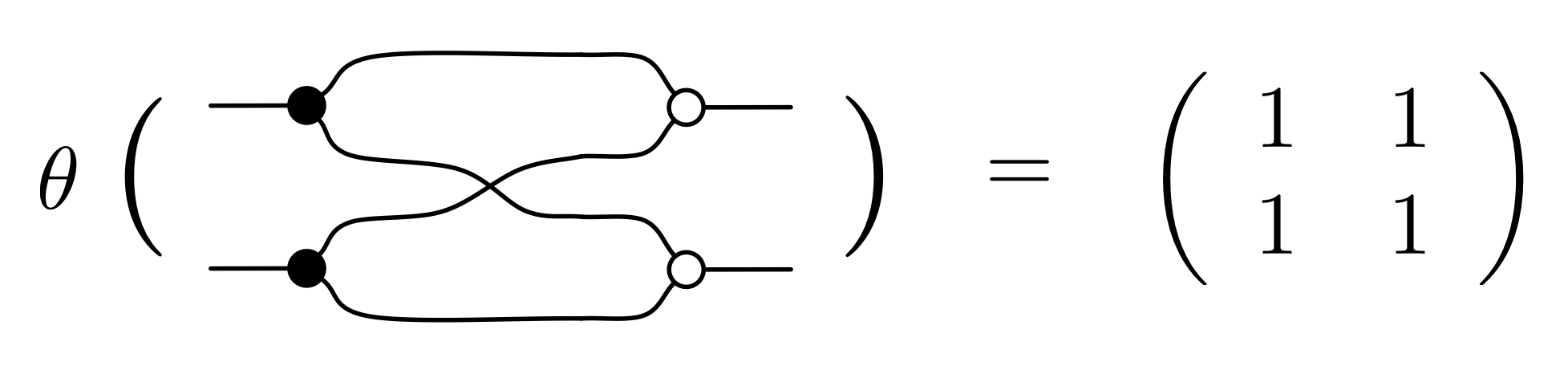
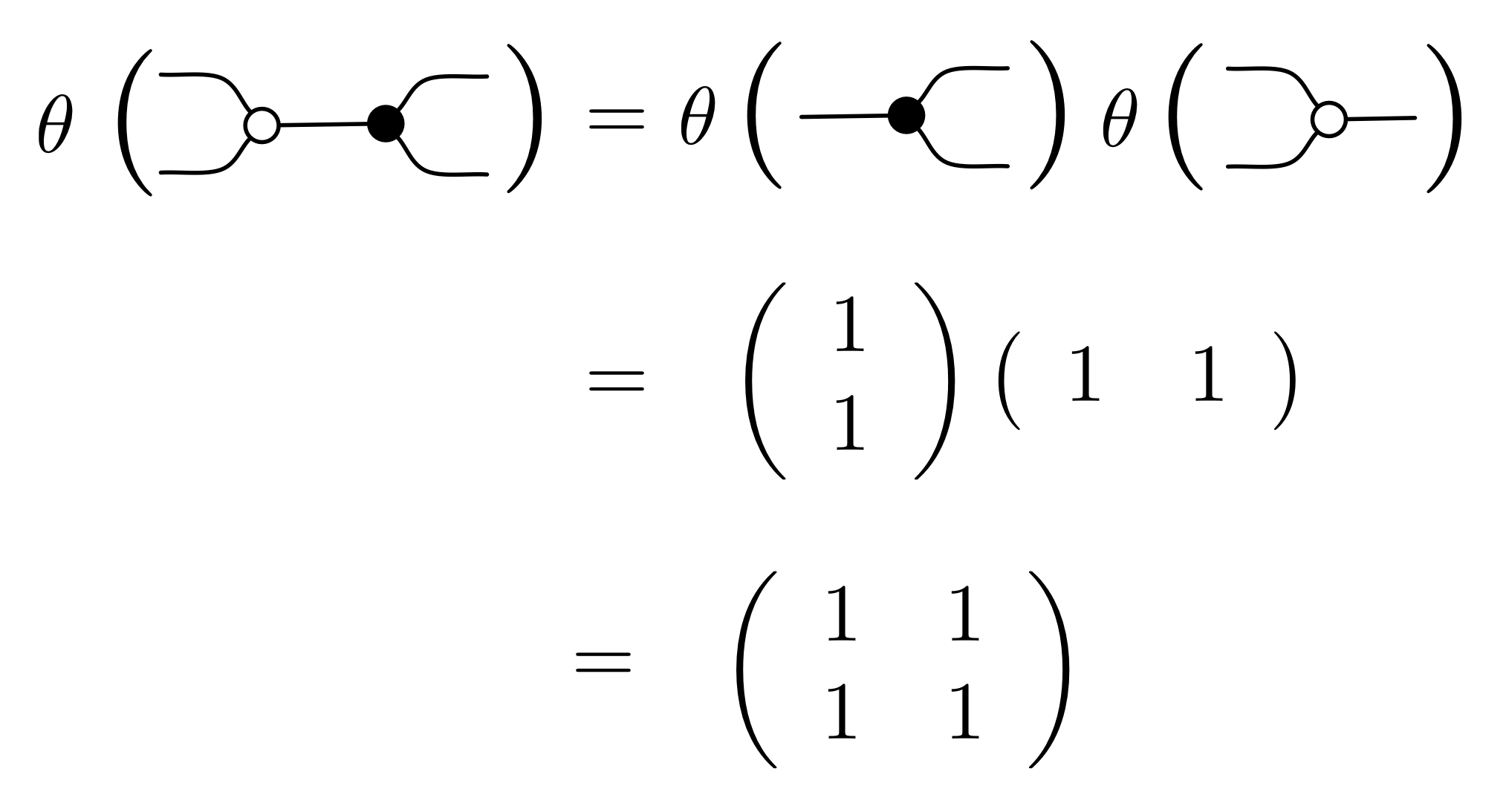
For point 3, for now I’ll just tell you what the relation for the twist 2 → 2 is and hope that it gives you the general idea. The twist in LinRel is the smallest linear relation that contains the elements

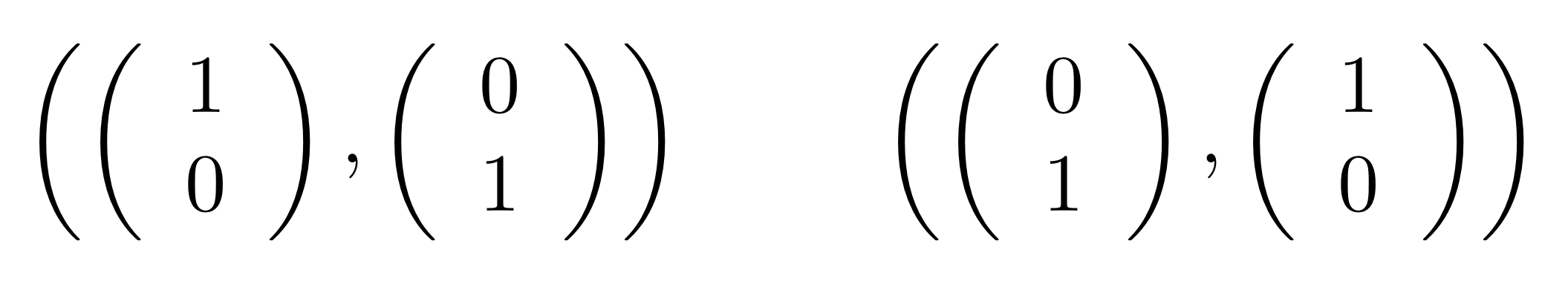
Since we need to close under addition and scalar multiplication, elements in this relation will look like

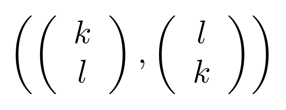
where k and l are fractions.

We have already discussed the relational semantics of the generators in Episodes 22, 23 and 24 and verified that the equations make sense, relationally speaking. It is not difficult to check that each of the relations is linear. Long story short, this assignment of relations to generators defines a homomorphism of props

IH → LinRel.

As we will eventually prove, this is an isomorphism; it is both full and faithful.

The proof of IH ≅ LinRel is quite a bit more involved than the proof B ≅ Mat and H ≅ Mat_Z. We will eventually go through it in detail—apart from following our principle of not handwaving, the proof is quite informative. But for now, LinRel and its diagrammatic presentation IH are perfect playgrounds for linear algebra and that’s what we will concentrate on over the next few episodes.

In the last episode we discussed how (1, 1) diagrams allowed us to divide by zero. By looking at the corresponding situation in LinRel, we can shed some more light on this curiosity. So let’s take a look at linear relations Q ⇸ Q: since IH ≅ LinRel these are in 1-1 correspondence with (1, 1) diagrams. We can plot linear relations of this type using conventional graphical notation, thinking of the domain as the horizontal x axis and the codomain as the vertical y axis.

Since every linear relation must contain the pair that consists of zero columns, every plot will contain the point (0,0). In fact, the singleton {(0,0)} is itself a linear relation: clearly it satisfies the two required properties. Here’s its plot.

The diagram for this linear relation is

which we dubbed ⊥ in the last episode. Next up, the entire set Q×Q is a linear relation. Here we colour the entire plane red. Sorry for the eye burn.

The corresponding diagram is

which we were calling ⊤ last time. These two linear relations give some justification for the names ⊥ (bottom) and ⊤ (top), since the former is—set theoretically speaking—the smallest linear relation of this type, and the latter is the largest.

The other linear relations are all lines through the origin. So, for example, the plot for the identity diagram

is the line with slope 1.

All the fractions arise like this. For example, the line for the fraction –¹/₂, diagrammatically

is the line with slope –¹/₂

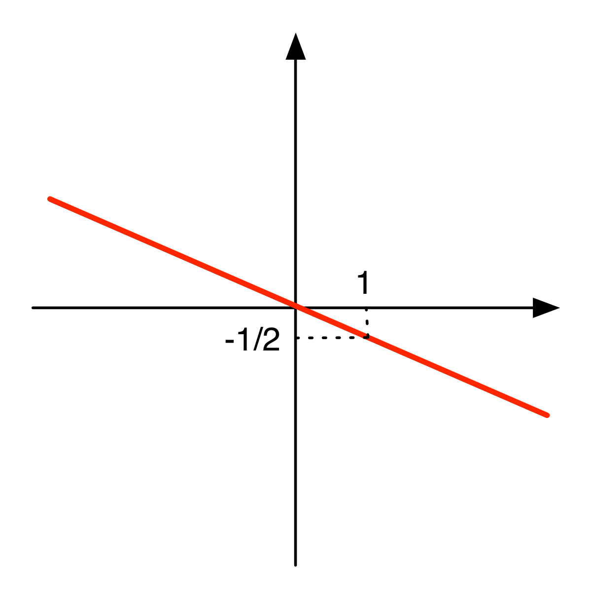
You get the idea for the other fractions.

There are two lines that represent interesting corner cases. The first is the line for 0

which is the line with zero slope, that is, the x-axis.

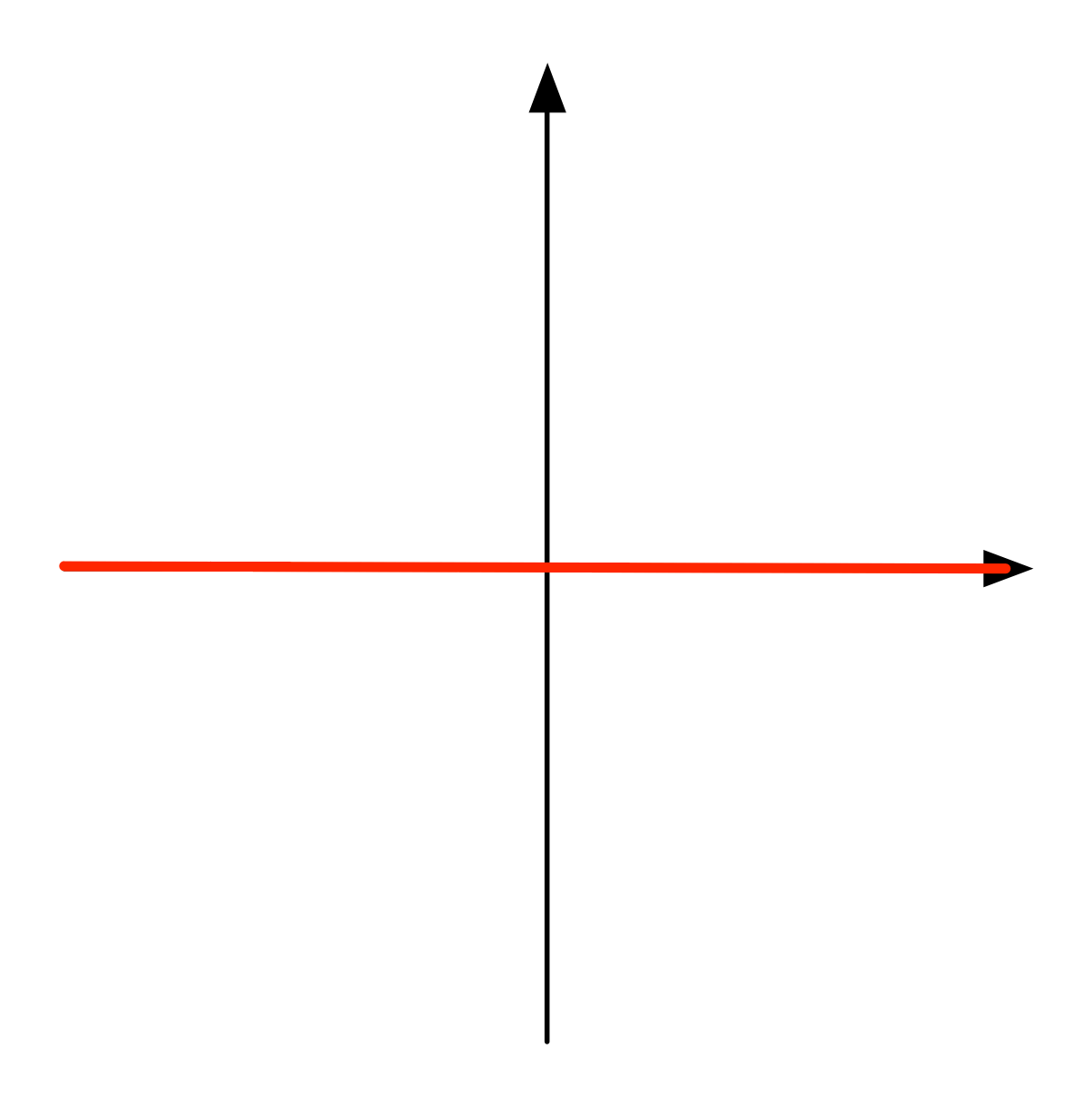
Finally, there’s the line with “infinite” slope, the y-axis.

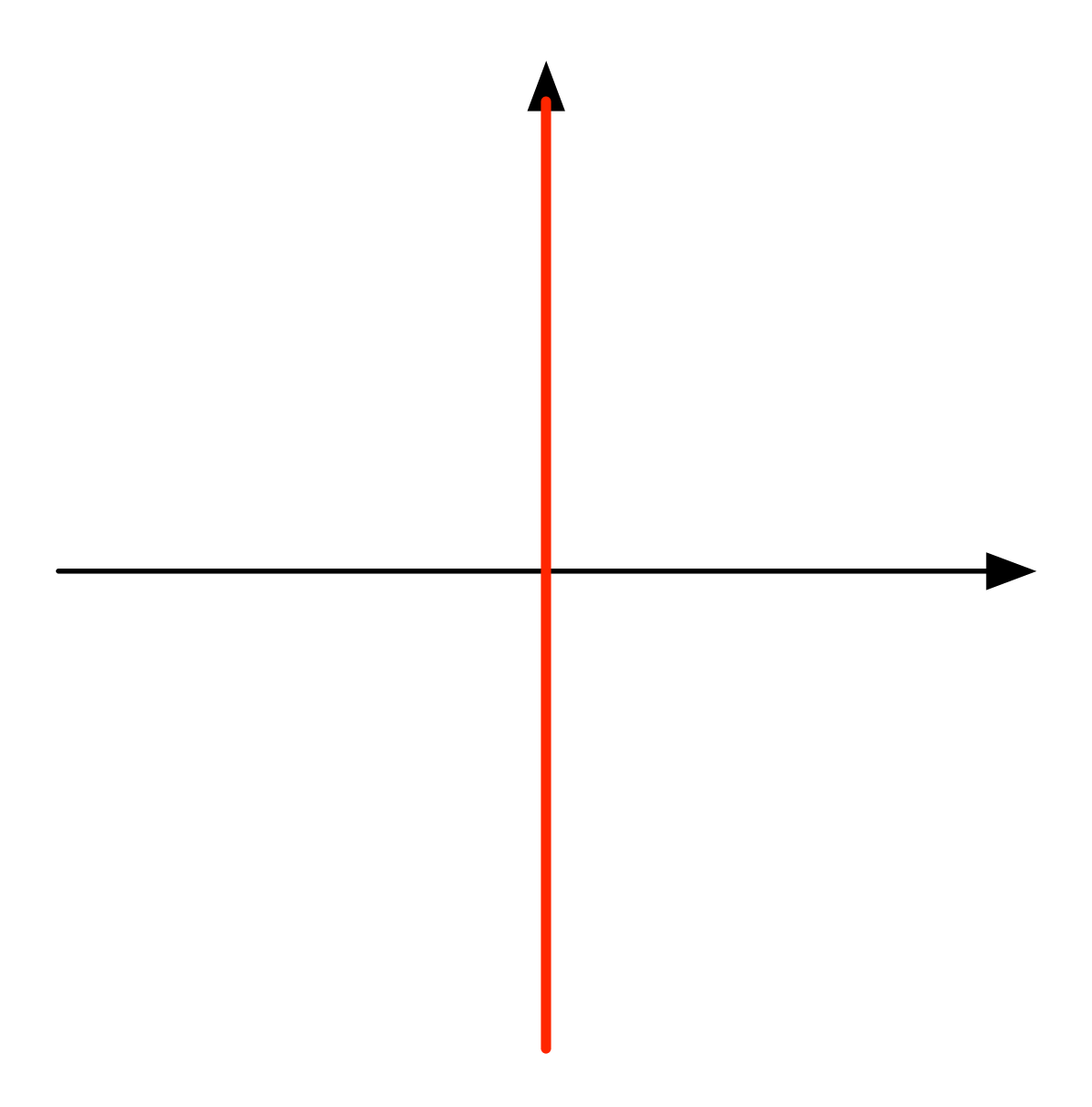
which is the plot for

that we called ∞ in the last episode.

If we think relationally, then the operations x+y, x×y and ¹/_x are all easy to define, and are total on the set of linear relations Q ⇸ Q. Multiplication is simply relational composition, and ¹/_x is the opposite relation x^†. Finally, addition can be defined set theoretically as

x + y = { (a, c) | there exist (a, b1) in x and (a, b2) in y such that b1+b2 = c }.

The above definition simply mimics the sum operation, as we have been doing with diagrams. So we could reconstruct the addition and multiplication tables from the last episode by working directly with linear relations.

Identifying numbers with lines through the origin is an old idea. It is one way to understand projective arithmetic. What is not so well-known is that we can define the arithmetic operations directly on the underlying linear relations, and moreover, throwing ⊤ and ⊥ into the mix makes the operations defined everywhere, with no need for dividebyzerophobia. If you have seen this done somewhere else, please let me know!

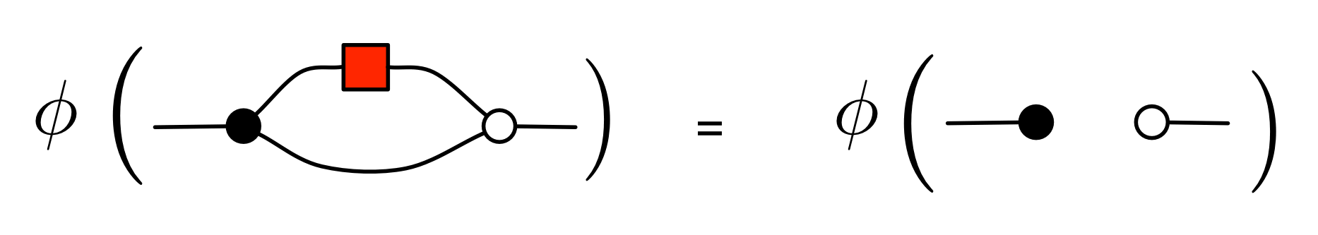
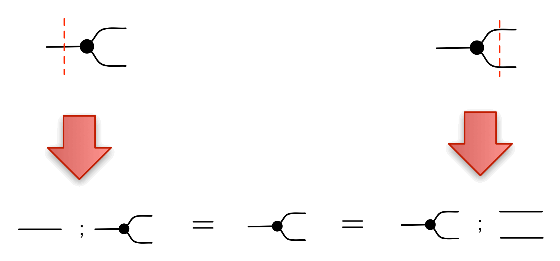
Here’s one very cool fact about LinRel, and it concerns the mirror image symmetry †. Remember that if R is a relation then R^† is the opposite relation: (b, a) is in R^† exactly when (a, b) is in R. In the last episode we saw that for any (1,1) diagram d we have

d;d^†;d = d.

It turns out that this works for arbitrary linear relations. Thus R^† is always the weak inverse of R. This is something that will be very useful for us in the future. Let’s prove it.

Suppose that D is some linear relation. Since D;D^†;D and D are both sets (of pairs), to show that they are equal it’s enough to show that each is a subset of the other. It is easy to show that every element of D must be an element of D;D^†;D, since, taking (a,b) in D, the chain of elements (a,b), (b,a), and (a,b) proves that (a,b) is in D;D^†;D.

We just need to show that the opposite inclusion also holds. So suppose that (a, d) is in D;D^†;D. By definition, there are b, c such that (a, b) is in D, (b, c) is in D^† and (c, d) is in D. And since (b, c) is in D^†, (c, b) is in D.

Now, using the fact that D is a linear relation that contains (a, b), (c, b) and (c, d), we have that

(a, b)-(c, b)+(c, d) = (a–c+c, b–b+d) = (a, d)

is in D.

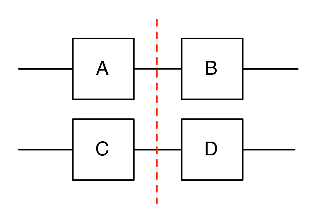
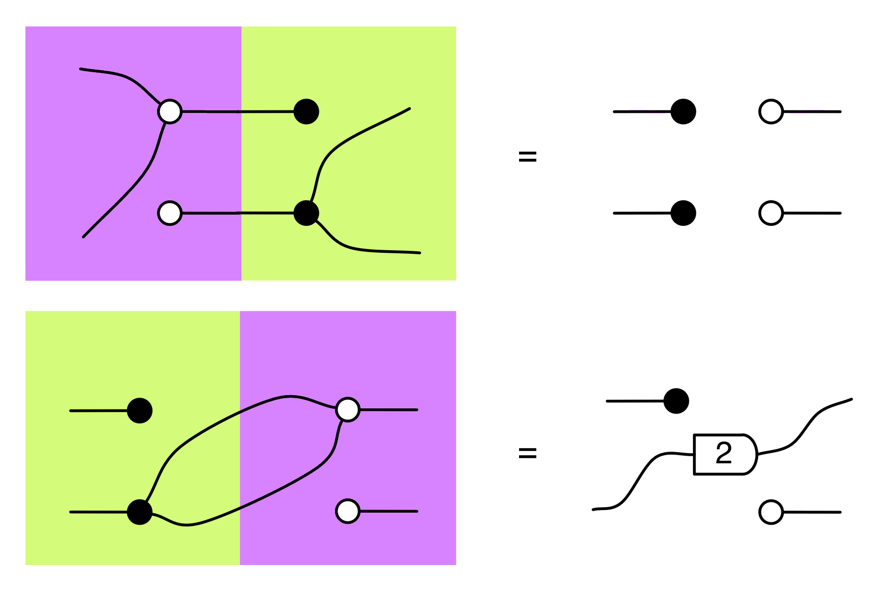
The fact that D;D^†;D is not larger than D is one thing that’s special about linear relations: it is not true for ordinary relations! For example, think about what happens to this relation 2 ⇸ 2:

Today is Boxing Day, so this is a Christmas special episode of the blog. The next one will probably arrive in January, so let me take this opportunity to wish everyone a fantastic

Continue reading with Episode 28 – Subspaces, diagrammatically.

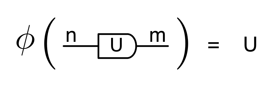
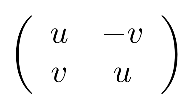
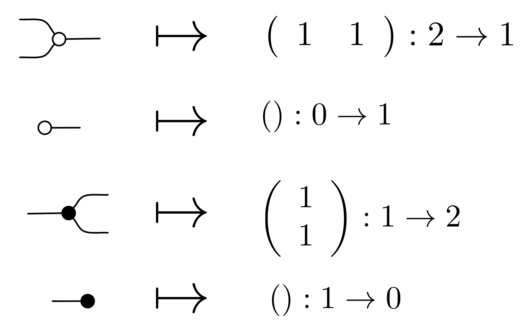
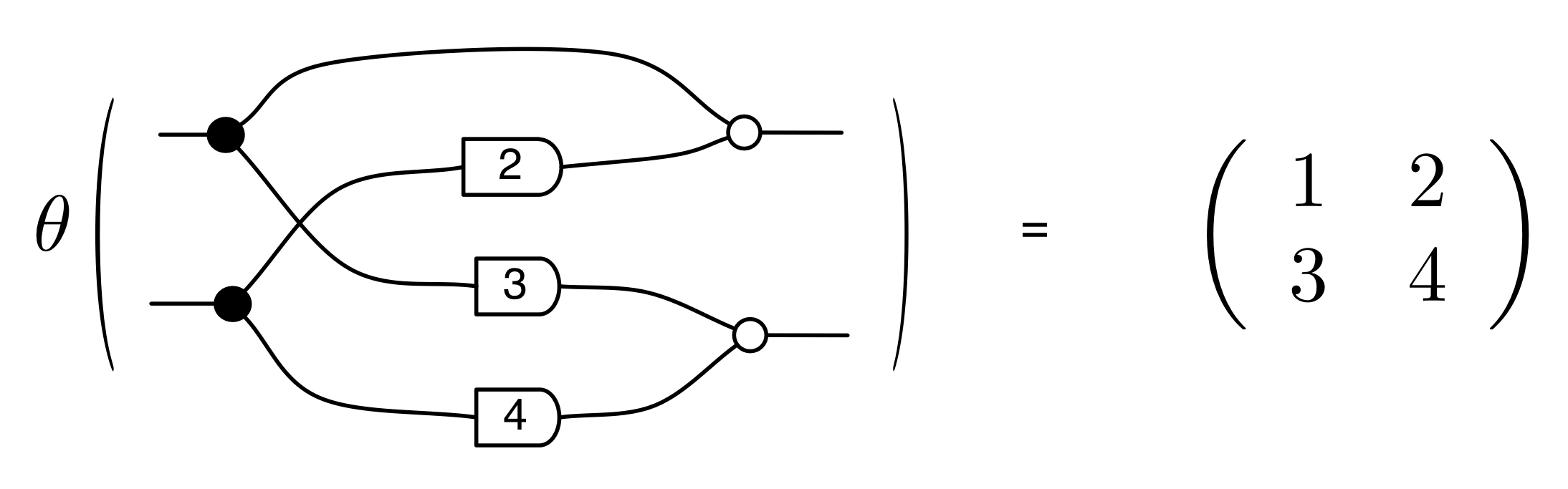
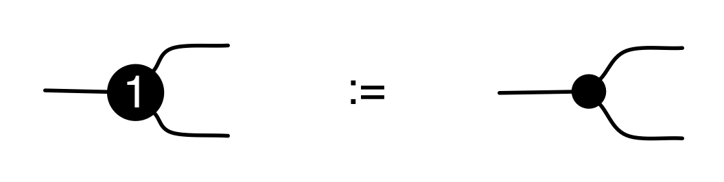
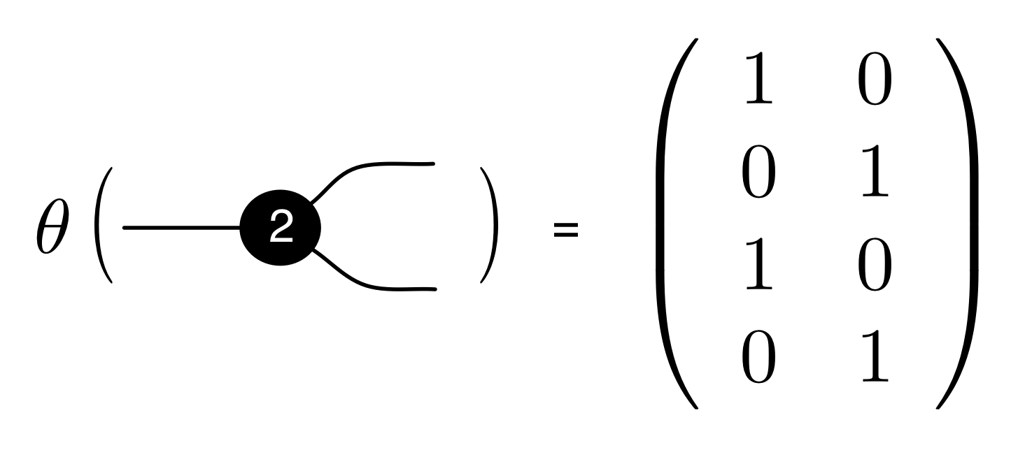
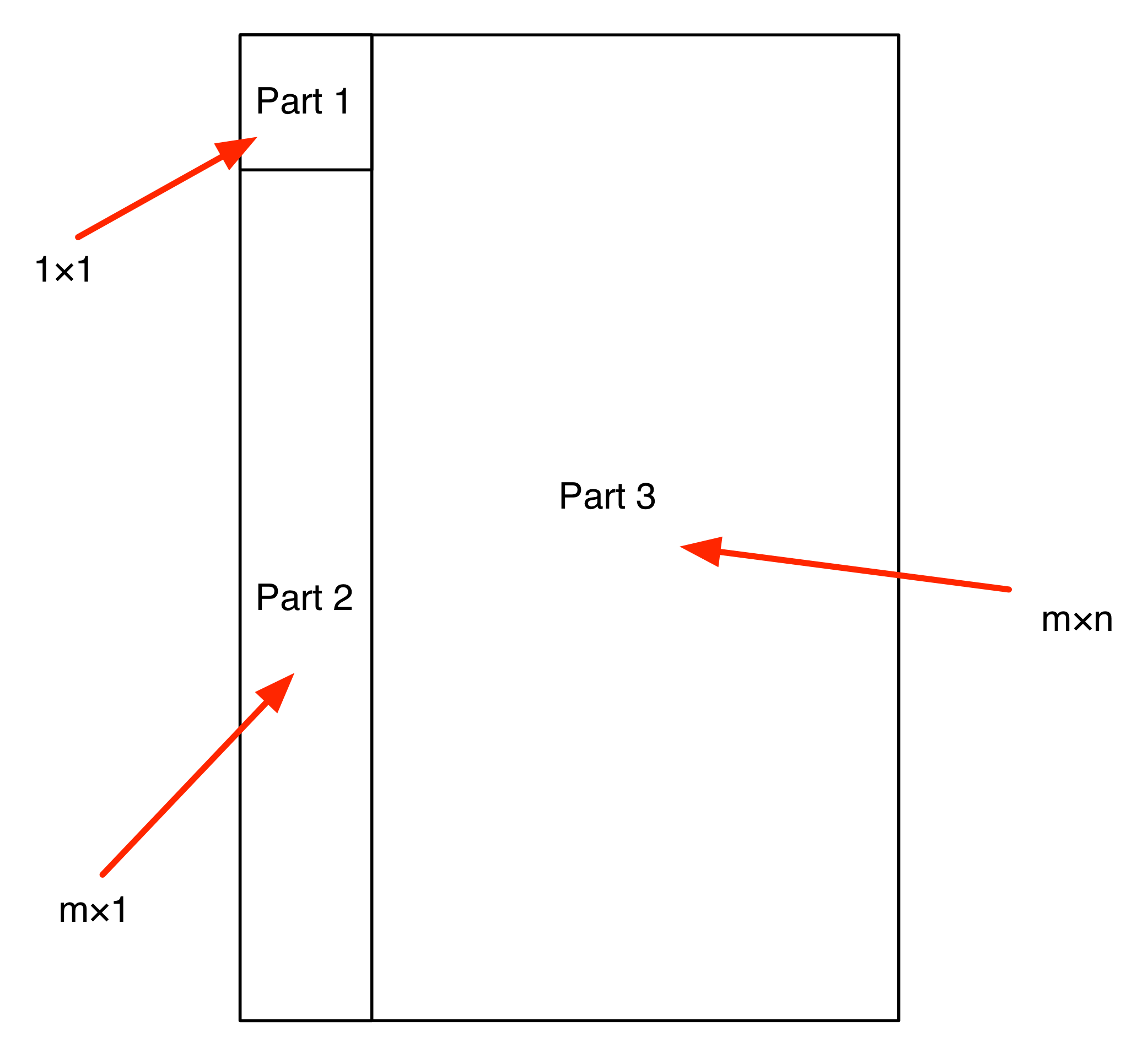
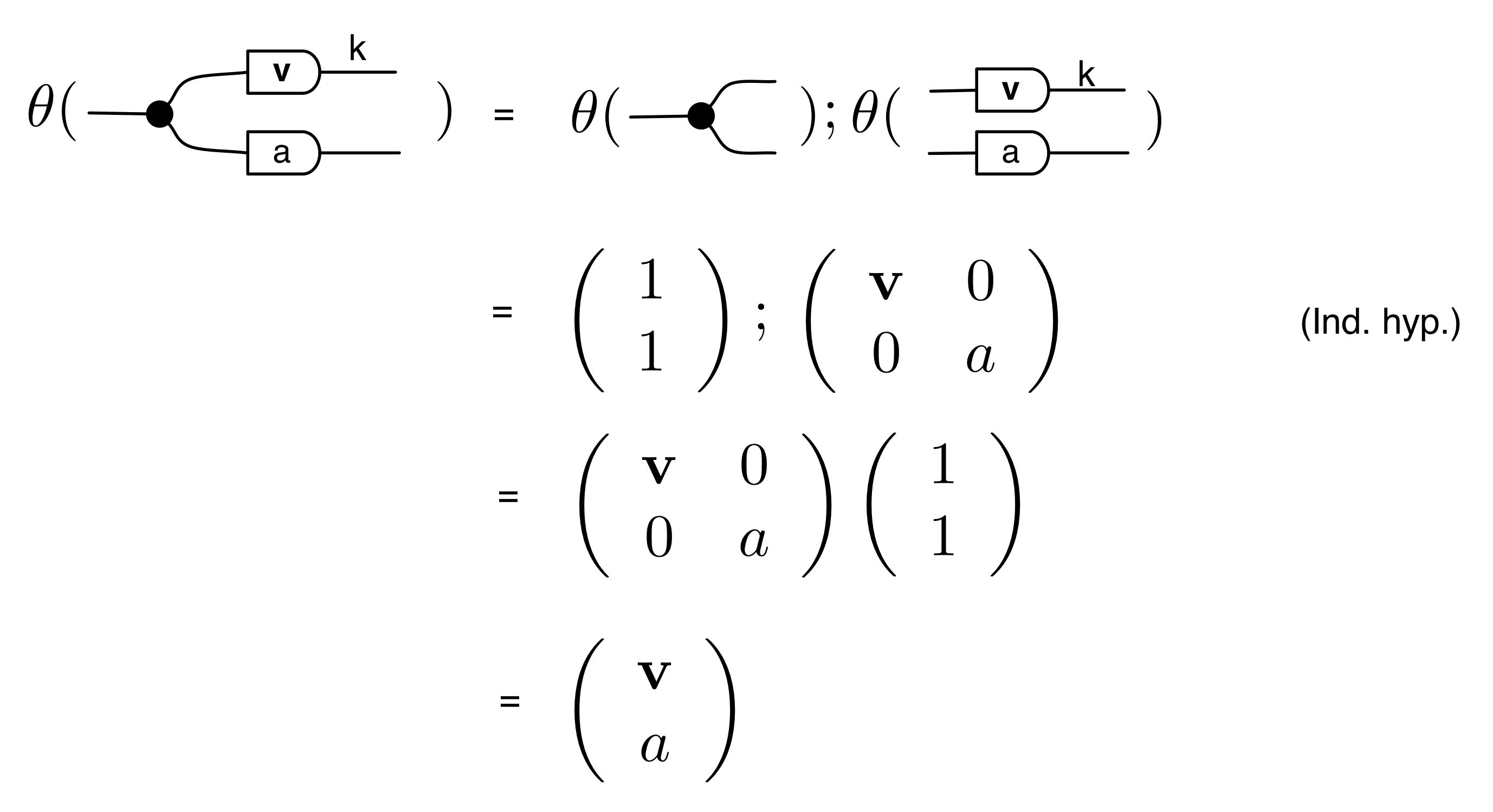
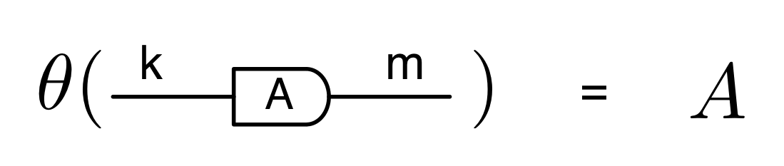
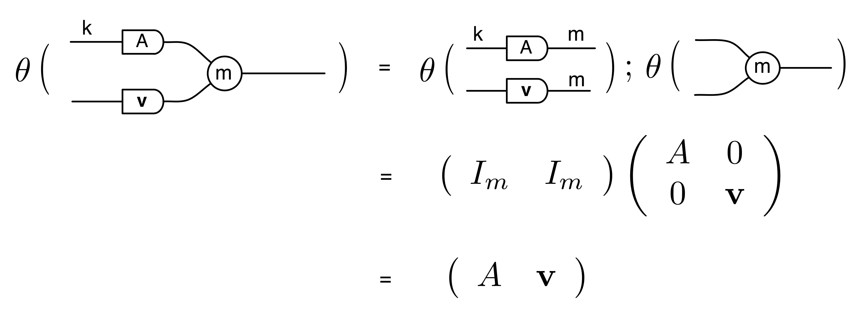
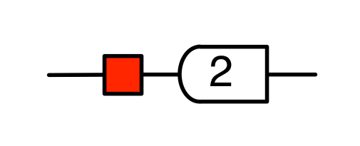
19. Integer Matrices

In the last episode we introduced the fifth and final principal actor of graphical linear algebra, the antipode. This episode’s main task is showing that diagrams built up of the five generators constitute a diagrammatic language for integer matrices and their algebra. We will also discuss a cute example involving the complex numbers.

The cheat sheet for the diagrammatic system H that includes the antipode is repeated below for easy reference.

We have already showed that H allows us to extend the syntactic sugar for natural numbers to a sugar for all the integers. We have also verified that the integer sugar obeys the usual algebraic laws of integer arithmetic. In particular, we proved that

using the equations of H and diagrammatic reasoning: this is just -1 ⋅ -1 = 1, expressed with diagrams.

Let’s start with an example. The diagram below has two dangling wires on both sides.
As such, it ought to denote some 2×2 matrix, and to get the entry in the ith row and jth column we need to look at the paths from the jth dangling point on the left to the ith dangling point on the right.

Before the antipode entered the frame, it sufficed to count the number of paths; the current situation is a little bit more complicated because there are positive paths—those on which the antipode appears an even number of times—and negative paths, those with an odd number. To get the relevant integer entry, we need to take away the negative paths from the positive paths. So, in the very simple example above, we have exactly one positive path from the first point on the left to the second point on the right, and one negative path from the second point on the left to the first on the right. The corresponding matrix is therefore:

Actually, I didn’t choose this matrix at random: it allows us to consider the complex integers (sometimes called the Gaussian integers) and their algebra in a graphical way. We will come back to this after tackling the main topic for today.

We want to prove that H is isomorphic to the PROP Mat_Z of matrices with integer entries. The letter Z is often used to mean the integers, from the German word Zahl meaning number; this notation was apparently first used by Bourbaki.

Mat_Z is similar to the PROP Mat that we discussed in Episodes 12 and 13: the arrows from m to n are n×m matrices, and just like before composition is matrix multiplication. The monoidal product is again direct sum of matrices.

The proof H ≅ Mat_Z(the symbol ≅ is notation for isomorphic to) is similar, and not much more difficult than the proof, outlined in Episodes 15 and 16, of B ≅ Mat. Let’s go through the details.

First we define a homomorphism of PROPs from H to Mat_Z. Let’s call it φ, the Greek letter phi. Since both H and Mat_Z are PROPs, and H is a free PROP built from generators and equations, it is enough to say where φ sends all the generators, and then check that the equations of H hold in Mat_Z.

It turns out that φ works the same way as θ for all of the old generators. The new part is saying where the antipode goes, and not surprisingly, it is taken to the 1×1 matrix (-1). Like so:

For φ to be well-defined, we need to check that all the equations of H also hold in Mat_Z. Fortunately, most of that work was already done for θ, we only really need to check the new equations that involve the antipode. Let’s check the most interesting of these, (A1); we need to calculate whether the following is true:

This amounts to checking if

and it does, indeed, work. The other equations, (A2) through to (A5) are similarly easy computations and we will skip them; but feel free to check!

So we have a homomorphism φ: H → Mat_Z. To show that it is an isomorphism, we will show that it is full and faithful. Fullness—the fact that every matrix has a diagram that maps to it via φ—is the the easy part.

First, we need to check that the sugar that we defined in the last episode works with φ as expected, which is confirmed by the following simple calculation:

Any matrix with integers as entries can now be constructed following the procedure described in Episode 15. We will skip the details, as it is all pretty straightforward! The upshot of the construction is that we can extend the sugar for natural number matrices to a sugar for integer matrices: given an m×n integer matrix U we obtain a sugar

such that

This establishes that φ is full.

So what about faithfulness, the property that says that whenever two diagrams map to the same matrix then they must already be equal as diagrams?

The trick is to get our diagrams into the form where the

copying comes first, then the antipodes, then the adding (★)

One way of doing this is to use the theory of distributive laws. Eventually we will go through all of this properly, but for now I will just give you a high-level executive overview. The main insight is that we have three different distributive laws, the first involving the adding and the copying (B1)-(B4), the second the antipode and copying (A2)-(A3), and the third the antipode and adding (A4)-(A5).

The three distributive laws, are compatible with each other in a sense identified by Eugenia Cheng in her paper Iterated distributive laws. The fact that the distributive laws play together well in this way gives us the factorisation (★) that we want. We will discuss Cheng’s results in more detail in a later episode. Incidentally, she has recently written a book about category theory and recipes; I wonder if she knows about Crema di Mascarpone!

We could also try a rewriting argument, taking for granted that the rewriting system described in Episode 16 terminates. Adding the following rules

it seems that the expanded system ought to terminate also, although I have not yet got around to proving it. These termination proofs are always really messy for a rewriting amateur like me; I would love to hear from an expert about how to do these kinds of proofs in a nice way.

Once we know that every diagram can be put in the form (★), the proof of faithfulness is fairly straightforward. We start with those diagrams that have one dangling wire on each side. Every such diagram in the form (★) is either the sugar for 0 (a single discard followed by a single zero) or it can be rearranged into the form:

for some natural number k of wires with one antipode and some natural number l of wires with no antipode. This is because we can always get rid of redundant discards and zeros with (Counit) and (Unit), cancel out multiple antipodes in series using (†), then rearrange, and eat up any annoying permutations with the iterated copy and add sugars.

Once our diagram is in this form we can desugar and repeatedly use (A1), each time destroying one pair of antipode wire and no-antipode wire. Either we end up with no antipodes left, in which case the diagram is equal to a non-negative sugar, or we end up with some number of antipode wires. In the latter case, we can use (A2) to pull out the antipode to the left, obtaining the sugar for a negative integer. We have thus shown that faithfulness holds for the (1,1) case, since every such diagram is equal to some integer sugar.

The general case, where diagrams can have any number of wires on the left and right, comes down to transforming the diagram in matrix form, as explained in Episode 16. This step completes the proof that φ is faithful, and since we already know it is full, it is an isomorphism.

So far we have been identifying “numbers” with diagrams of a particular kind; those with one dangling wire on each end. In B this gave us the natural numbers, and in H it gives us the integers. But, as argued in Episode 17, there’s nothing particularly special about (1, 1) diagrams; well, maybe apart from the fact that both in B and H composition for (1,1) diagrams turns out to be commutative. Our obsession with the (1, 1) case is due to history—the traditional way of doing matrix algebra means the concept of ‘number” comes first, then the concept of “matrix”.

The complex numbers are a nice example where it makes sense to consider “numbers” as something different than (1,1) diagrams A complex number can be written as an expression r + si where r, s are numbers and i is a formal entity that behaves like a number, but with the mysterious property i²= -1. The numbers r and s are sometimes called, respectively, the real component and imaginary components. What is important for us is that to describe a complex number, it suffices to keep track of two ordinary numbers. Our intuition is that wires carry numbers, so it makes sense to carry a complex number with two wires, the first for the real piece, the second for the imaginary piece.

Now if we multiply a complex number r + si by i, we get (r + si)i = ri + sii = -s + ri. So what was the real component becomes the imaginary component, and the negative of what was the imaginary component becomes the real component. We have a diagram for that, and we have already seen it in this episode:

It thus makes sense to call this diagram i:

Now if we multiply r + si by an integer u, we get (r+si)u=ru + sui. So both the components are multiplied by u. We also have a diagram for that:

where on the right hand side we used the sugar for integers from the last episode.

For the rest of this section, to stop the proliferation of the digit 2 that clutters the diagrams, we will just draw the 2 wire using a thicker line, like so:

Now we can do some calculations. First if we compose the diagram for i with itself we get:

We can also show that i commutes with integers:

Following the general pattern of this blog, we can ask what kinds of diagrams one can construct using the following gadgets.
Using our standard box of tricks for reasoning about diagrams, it is not difficult to show that the diagrams with one thick wire on each side will, in general, be of the form:

Composing two such entities gives us

which is of course what you’d get if you multiplied out two complex integers (those complex numbers u+vi where u and v are integers). In general, the diagrams that can be constructed from bricks (‡) are matrices with complex integer entries.

So what exactly is going on here? Let’s take a look under the hood.

The result is in matrix form, and corresponds to the 2×2 matrix:

and this is known as one way of representing complex numbers using matrices.

There is one more interesting thing to say here. Let’s take a look at the bizarro of i.

So the bizarro of i is -i. It follows that the bizarro of a general diagram constructed in the system (‡) corresponds to the operation known as conjugate transpose in complex matrix algebra.

If you know about quaternions, they can be considered in a similar way. Of course, we are constrained to integer coefficients for now. Not for long ☺.

I will give a 3 hour tutorial about graphical linear algebra at QPL ’15 in two chunks on Monday and Tuesday of next week. I’m desperately trying to get the slides done on time. Running this blog has been helpful in that it forced me to develop material, but unfortunately what we have covered so far will only be enough for around the first 30 mins; I should have started this blog back in January!

Continue reading with Episode 20 – Causality, Feedback and Relations.

17. Maths with Diagrams

The discussion over the last few episodes has now led us to the point where we have two different languages to talk about the same thing. The two languages, however, are rather different. One consists of diagrams, the other of matrices populated with natural numbers. If you already knew about matrix algebra, maybe you’re asking yourself the question “What’s the point of all these diagrams then? They don’t tell me anything that I didn’t know before. Is this guy claiming that this diagrammatic language is better in some way?”

The short answer is no. I don’t want anyone to throw away their matrices: there are extremely good reasons to know and care about them. But I have two arguments for why we should also care about diagrams.

The first argument is that a different language means thinking about the conceptual landscape in a new way. We will see this over and over again in graphical linear algebra, and sometimes it will cause us to reevaluate certain dogmas: ways of doing things that have come about because of the way that the standard notation works, rather than real underlying mathematical issues. These kind of things are not easy to spot if you only know one notation.

More generally, the idea that the languages we use influence how we think and act—linguistic relativity if you will—is well-known and appreciated by programmers. Most programming languages are Turing complete and so have equivalent power. So why not just learn one, say x86 assembly, and stick with it?

Programmers deal with real problems, which usually do not involve writing functions to compute the Fibonacci sequence or, infamously, inverting a binary tree. Real problems are multi-faceted, and for some parts it may be useful to put on a functional hat, for others an object-oriented hat, and so on. The different ways of thinking that the various programming methodologies bring to the table are appreciated because

complex problems benefit from a combination of approaches.

When I was a student in the 90s that there were many entertaining flame-wars about which programming language approach was the best. As with most flame-wars, they were pretty pointless: programming has since grown up and nowadays it’s very rare to hear somebody claiming that a particular way of doing things is intrinsically better than another. Good programmers are comfortable thinking in several different languages, and choose the one that is most suitable for the current (sub)problem at hand. Flexibility is key.

Because of this, in the last 10 years or so, the boundaries between different language families have been blurring. For example, most functional programming languages have clever ways to do imperative things, and conversely, more and more functional features are making their way into industrial strength imperative languages. It’s pointless to argue which is the best approach, or the best language: such a thing doesn’t and will never exist. And anyway, it’s fun to see how your favourite problems can be solved with some newfangled language!

It’s been really interesting to see how different communities have reacted to this blog. About a month ago somebody posted a link to this blog on Hacker News. That link made it to the front page and resulted in a massive amount of interest, which really surprised me… who knew that so many people cared about linear algebra! Last week I posted a link there myself and again the feedback has been really great. I’ve also been regularly posting links on Reddit’s /r/math, which has also resulted in a lot of really interesting and useful comments, but also quite a bit of skepticism and maybe even a touch of hostility.

Allow me to philosophise for a moment for why this is the case. I think that it’s because many mathematicians are just not used to the idea of having different languages to talk about their concepts. In many mathematical subfields the notation is very conservative and standardised. It has evolved so slowly, so imperceptibly, that mathematical culture almost brings with an an understanding that “standard notation” has been given to us by some higher power and it is not to be disturbed. Anyway, the concepts are the important things so who cares about notation. Many mathematicians simply don’t see the value in exploring different ways of expressing themselves. Programmers, it seems, are much more receptive to the idea.

The second argument for why we should care about diagrams is Occam’s razor — the idea that one should trim the fat: discard unnecessary assumptions to try to get at the core of problems. So let’s consider the amount of intellectual technology necessary to develop the concept of

matrices of natural numbers, and their algebra ①

I need you to forget for one moment that you know all of these things already and that they are totally obvious to you; let’s pretend, for one moment, that we are explaining Earth mathematics to a group of interested Martians. And let’s not be too creative about the Martians. Let’s assume that they are of the Star Trek variety: three dimensional and humanoid enough to interest Dr McCoy in extra-curricular activities, but without the experience of an Earth education. So, to make them understand what ① means, we need to:

Explain the concept of natural numbers, together with addition and multiplication
Show that the natural numbers form what is called a commutative semiring. Let’s go through these requirements:
1. addition is associative, commutative, and has 0 as it’s identity; that is, for any natural number n, we have 0 + n = n = n + 0
2. multiplication is associative, commutative and has 1 as it’s identity; that is, for any natural number n, we have 1· n = n = n · 1
3. multiplication distributes over addition, that is, for all natural numbers a,b and c, we have a·(b + c) = a·b + a·c (in a non-commutative semiring we would also require (b+c)·a = b·a + c·a, but that follows here from commutativity of multiplication)
Define the concept of an m×n matrix, a grid of numbers. If we are totally honest then we ought to probably also go through the corner cases where any combination of m and n can be 0.
Write down the formula for matrix multiplication. This relies on already knowing about addition and multiplication of natural numbers. The semiring properties are necessary for matrix multiplication to behave as expected (e.g. for it to be associative).
Write down the formula for matrix addition.

This is actually a significant amount of work. And maybe the Martians are a bit curious about where exactly did the formula for multiplying matrices came from. They know from previous Earth experience that you can’t really trust those pesky humans and their crazy ideas.

On the other hand, we have already done all of the work of showing how diagrams work in the first few episodes of this blog. If explaining to the Martians, we would need to:

Explain the idea of magic Lego; the algebra of diagrams that consists of the two operations of direct sum ⊕ and composition ;
Go through the rules of diagrammatic reasoning: stretching, tightening, moving generators along wires
Introduce the four generators together with the ten equations.

Let’s compare the two ways. In the traditional approach, one first defines the natural numbers and then “bootstraps” matrices on top. With diagrams, there is no precedence given to natural numbers as such; everything gets defined at the same time. Natural numbers can be recovered as special kinds of diagrams, those with one dangling wire on each end. We don’t need to invent any extra formulas for multiplying matrices because composition is a basic operation of the algebra of diagrams. Matrix addition is not a primitive operation at all, it can be constructed from the diagrammatic primitives.

Having said all that, this blog so far has followed a rather conventional route: first we talked of natural numbers as diagrams and then of matrices as diagrams. Today, we are going to go back and think about how the maths would have been developed without knowing about natural numbers and matrices from the outset. We will rediscover diagrams by focussing on the operations and constructions that are natural in their language and see where that takes us.

To spice things up let’s try some alternate history. This is something that historians really hate; my sister, who is a historian, always gets annoyed when I bring it up. But who doesn’t love to annoy their siblings?

We need to turn the clock back to before matrices were common, before notation settled into what appears in textbooks today. Our story thus takes place in early 13th century Pisa. Our hero is a certain young man, Fibonchi, a contemporary and friend of Fibonacci.

While a teenager, Fibonchi sailed to the Balearic Islands with a Pisan trade fleet. In Palma, he met a wise old Berber merchant who introduced him to four curious operations that spoke of putting things together and copying them, governed by collection of simple, self-evident rules. The old men of Palma enjoyed drawing the diagrams and even used them to perform some calculations.

On his way back home, Fibonchi realised that the diagrams are what is now known as a recursive data type: every diagram is put together from the four simple bricks, the identity and twist. Using this insight, he was able to prove a number of interesting things about them, using the principle of induction.

To help in his calculations Fibonchi wrote down the formula for diagrams that copy and add not just one wire, but an arbitrary number on wires. Coincidentally, this was the syntactic sugar we discussed a couple of episodes back.

Next, Fibonchi proved that these sugars satisfied a very pleasing property with respect to arbitrary diagrams. For example, given any diagram D with m dangling wires on the left and n dangling wires on the right, the following is true:

Of course, once Fibonchi had finished this proof, he immediately wrote down his second theorem.

He did not even bother writing down a proof, since he was told about about the principle of “bizarro” by the old man in Palma. Because all the equations in the system have bizarro (reflected, colour-swapped) versions, once you proved a theorem you’ve also proved its bizarro cousin.

Fibonchi also noticed the following two related facts, the second the bizarro version of the first.

These properties intrigued Fibonchi, and he went ahead and defined an operation on compatible diagrams—those that agreed in their respective numbers of dangling wires on the left and right. He called the operation sum. This operation would be rediscovered in different notation a few centuries later and given the name matrix addition.

He proved that sum was associative

and commutative:

Moreover, each compatible family of diagrams contained an identity for this operation:

Fibonchi showed that D + 0_m,n = D = 0_m,n + D.

He also noticed that composition distributes over sum: we have

D ; (E+F) = D ; E + D ; F

The proof, reproduced below, was a straightforward application of his first theorem.

He was, of course, immediately able to state the bizarro version:

(D+E) ; F = (D ; F) + (E ; F)

Fibonchi knew that composition of diagrams was not commutative, in most examples it didn’t even make sense to compose diagrams in more than one way because the dangling wires did not match up. Non-commutativity was the norm. However, he did notice some peculiar things about diagrams with exactly one dangling wire on each end.

He noted that there was exactly one such diagram for every natural number, which gives the number of paths from the left dangling point to the right one. He understood that if two such diagrams have an equal number of paths then they are equal. His arguments were close to the rewriting argument of the last episode. Another strange thing was that the bizarro of every such diagram was equal to the diagram you started with.

Most curiously of all, composition between such diagrams was commutative, which Fibonchi confirmed with a simple induction. First the base case, where the first diagram has zero paths:

and the inductive step:

Inspired by Fibonacci’s masterpiece Liber Abaci, Fibonchi wrote his own treatise entitled Liber Diagrammatis. Unfortunately it is now lost; the last remaining copy fell into the hands of a Livornese fishmonger sometime in late 16th century, who used it to wrap his wares. The Livornese never much liked the Pisans or what they had to say.

Fortunately, we can continue Fibonchi’s story on this blog.

Continue reading with Episode 18 – Introducing the Antipode.

15. Matrices, diagrammatically

We have established that there is a homomorphism called θ from B, the PROP of diagrams, to Mat, the PROP of matrices. To do this, it was enough to say where θ takes the four stars of the story so far: the add, zero, copy and discard generators.

The task for this and the next episode is to understand why θ is an isomorphism—a perfect translation—and to show that a PROP homomorphism is an isomorphism, it is enough to show that it is full and faithful.

The intuition for why the translation works well was established all the way back in Episode 10. The idea is that a diagram with n dangling wires on the left and m on the right translates to a matrix with n columns and m rows. In that matrix, the entry in the ith row and the jth column of the matrix is the number of paths from the jth dangling point on the left to the ith dangling point on the right in the diagram. It’s not difficult to verify that this is exactly how θ works: for example we have the following:

Now, to show that θ is full, we just need to convince ourselves that every matrix has a diagram that translates to it.

In fact, this may already seem to be pretty straightforward, given what we know about paths. If I give you some matrix then—looking at the example above for guidance—you should be able to go away and draw a diagram that does the job. Still, intuition doesn’t always cut the mustard, so it’s worthwhile to spend some time doing this properly. That’s our task for today. The proof of fullness also provides us with new syntactic sugars that make the diagrammatic language even nicer to use.

In Episode 9 we saw how diagrams with one wire dangling on the left and one on the right can be identified with the natural numbers. By now we know a whole lot more about diagrams. Today we will see that the diagram for a natural number n translates via θ to the 1×1 matrix (n). The proof that θ is full is the continuation of this story, since it amounts to building up a diagram for any matrix of any size.

Before we launch into the proof, we need to introduce a new family of syntactic sugars, one for each natural number m. Their names are m-copy and m-addition, and, just like copy and add, one is the bizarro version of the other. We therefore only need to concentrate on thinking about one, since the story for the other is simply the bizarro version.

Our old friend, the copy generator, has a single dangling wire on the left, and our standard intuition says that it works by copying whatever value appears on that wire to its two wires on the right. But what if there are values arriving on two or more wires, and we want to copy all of them? For example, in the case of two wires we would need to construct a circuit that has two dangling wires on the left and four on the right that behaves as follows, for any numbers x and y:

We can wire up an such a diagram using two copy constructors and a twist: we copy the x and the y, obtaining two xs and two ys, then we swap an x and y. Like this:

It seems that it should be fairly straightforward to construct such a gadget for three wires, four wires, and so on, using only copy, identity and twist. This is the idea of m-copy, where m is a positive integer, and we will draw it like this:

The white m in the middle of the black circle refers to the number of wires being copied. The black ms on the wires are a sugar that we have already seen: they mean m stacked identity wires, or m-wires for short.

The picture of the sugar is a bit busy with all of those ms. We want to keep our diagrams looking sharp, so when we use m-copies we will typically be a bit lax with writing all of these numbers. Just keep in mind that whenever you see one, it has an m-wire dangling on the left, and two m-wires dangling on the right. One more thing: if you want to draw this sugar on paper and you don’t have access to white pens, feel free to write the number above the circle.

Let’s go ahead and define it, using recursion. The base case, m = 1, is just the copy generator.

Next, the recursive case is:

So, to copy k + 1 wires, we can copy the first k wires recursively, copy the last wire, and then we have to make sure that the dangling wires line up properly on the right, using σ_k,1. We have already seen the case m = 2, so here’s what the construction gives us for m = 3:If, unlike me, you have a good memory, you probably remember a different sugar for copy, which we introduced in Episode 10. There we chained several copies one after the other, obtaining a copy sugar that has one dangling wire on the left and several on the right. Both the sugars are useful, and it’s possible to use them together, but it is important not confuse them.

It’s interesting to think about the matrices that correspond to m-copy. So let’s take a look at the first two:

The pattern is becoming apparent: in general, it’s not difficult to show that for an m-copy, the corresponding matrix is formed by stacking two identity matrices of size m, as illustrated below.

Although we don’t strictly need this for our fullness proof, in the future it will be useful to know that m-copy satisfies the same kind of equations as ordinary (1-)copy. In particular, there is the m-version of (CoComm):

where the role of the twist is played by σ_m,m. The proof is a pretty straightforward induction, and we will skip it. Similarly, we can prove an m-version of (CoAssoc)

and an m-version of (CoUnit).

The left hand side of the last equation features a new, but very simple, sugar: the m-discard: this is simply m discard generators stacked on top of each other. For example, this last equation, when instantiated at m = 2, looks like this when de-sugared:

The bizarro version of the m-copy sugar will also come in handy for us. Just as addition is the bizarro copy, m-addition is the bizarro m-copy. Being bizarro, we do not need to define it from scratch since we can take the recursive definition of m-copy, reflect it and invert the colours. But let’s just understand what it means in terms of our intuition; for example, the behaviour of 2-addition is as follows.

Following our bizarro tradition, we will draw m-addition like this:

and, just as expected, m-addition satisfies the m-versions of the adding equations.

These are:

The last equation features m-zero, which similarly to the m-discard, is simply m zero generators direct summed together.

Finally, let’s think about the matrices that correspond to m-addition. We already know that bizarro in the matrix world means transpose matrix, so it’s not surprising that we have:

We are ready to prove that θ is full, that is, given any m×n matrix A, there exists a diagram D such that θD = A. Let’s first consider the corner cases: m = 0, n = 0 or both m = n = 0.

When m = n = 0, there is precisely one matrix with 0 columns and 0 rows, the empty matrix (): 0 → 0. Coincidently, there is a diagram with 0 dangling wires on both ends, the empty diagram. Both the matrix and the diagram are actually id₀ in their corresponding PROPs, so θ by definition takes the empty diagram to the empty matrix.

When n = 0, m ≠ 0, the diagram that does the job is the m-zero. Similarly, when n ≠ 0, m = 0, the diagram that does the job is the n-discard.

The interesting part of the proof concerns m×n matrices where m,n≥1. Our proof is divided into three parts, and each part is an induction. In Part 1 we will handle 1×1 matrices, next the column vectors (m×1 matrices) in Part 2, and finally in Part 3 matrices of arbitrary size (m×n). Each part uses the results of the previous parts.

Part 1

Let’s get started by showing that fullness holds for every 1×1 matrix. What we want to prove is that, for any natural number a, we have:

where the diagram in the left hand side is the our diagrammatic sugar for natural numbers, which was the topic of Episode 9.

We can prove it by induction on a, the base case is:

where, by definition of composition in the PROP Mat of matrices, we multiply the unique 1×0 matrix with the unique 0x1 matrix. The result is a 1×1 matrix, and following the formula for matrix multiplication, it is the empty sum. And the number you get after adding up zero things is zero. So far so good.

Now for the inductive step: let’s assume that the claim holds for a = k, and show it for a = k + 1.

In the first step we use the recursive definition of the natural number sugar, and in the next two steps we use the definition of θ. We use the the inductive hypothesis in the fourth step. Next we just perform the calculation in the PROP of matrices. That completes the job for 1×1 matrices.

Part 2

Using what we already know, we will show that every column vector, that is, every m×1 matrix has a diagram that maps to it via θ. Again we do it using induction, but this time on the height of the vector, m. The base case is 1×1 matrices, which we have established in Part 1.

So, let’s do the inductive step: supposing that fullness holds for k×1 matrices, we want to show that it holds for (k + 1)×1 matrices. The key observation here is that every such matrix looks like this:

where v is a column vector of height k and a is some natural number. Using the inductive hypothesis, we know that there exists some diagram (that we may as well call v) with one dangling wire on the left and k on the right, such that:

Using this inductive hypothesis and our result from Part 1, we can build a diagram for the larger column vector:

and this completes the job. So we now know how to construct diagrams for column vectors of arbitrary size.

Part 3

This final part concentrates on arbitrary m×n matrices. The induction, this time, is on n. The base case is m×1 matrices, and we found out how to deal with these in Part 2.

Now, assuming that we can construct diagrams for m×k matrices, we need to show that we can construct them for m × (k + 1) matrices. The observation that we can make here is that any such matrix looks like this:

where A is some m×k matrix and v is a column vector tacked on at the end. The inductive hypothesis tells us that we have a diagram that translates to A:

and we can use this to construct a diagram for the larger matrix. To do this, we make use of the m-addition sugar that we cooked up before and the fact, shown in Part 2, that we know how to get a diagram for v.

That completes the proof: θ is full, as advertised.

Back in Episode 9 we introduced a syntactic sugar for natural numbers as certain diagrams. The proof of fullness shows us how to extend this to a sugar for any m×n matrix.

This means, that given a m×n matrix A, we have a diagram

We can reinterpret the induction proof, working back from Part 3 to Part 2, to obtain a recursive definition for this sugar, extending the natural number sugar of Episode 9:

This sugar will be quite useful for us as we do more graphical linear algebra, since it will allow us to consider any matrix of natural numbers as a diagram!

Continue reading with Episode 16 – Trust the Homomorphism, for it is Fully Faithful

13. PROPs (Part 2) and Permutations

First, a brief reminder of where we are at the moment. We are going through the various parts of mathematical structures called PROPs (product and permutation categories). As we go through each new piece, we pause to check that both our diagrams as well as matrices of natural numbers satisfy the conditions. The goal is to conclude that both diagrams and matrices organise themselves as the arrows of two PROPs. The translation from diagrams to matrices from two episodes ago will turn out to be an isomorphism of PROPs, which means that for all intents and purposes we can regard diagrams and matrices as different languages to talk about the same thing.

In the last episode we went through some of the structure of PROPs, but the story is not yet complete. Actually, so far we have talked only about the “PRO” in PROPs. The final P stands for permutation, and permutations are the main topic for today.

Let’s start by introducing another convenient syntactic sugar for diagrams. It will be useful for discussing permutations, but it will also come in handy for us later on. This one is pretty simple: whenever we write a natural number k above a wire, it simply means the diagram that results from stacking k copies of the identity on top of one another. Of course, when k = 1 there is no need to write any number at all: the wire with 1 above it is just a wire.

In the last episode we have seen that this diagram serves as the identity on k in the world of diagrams. There’s one thing to keep in mind about this sugar: it’s important not to confuse it with our standard intuition of numbers travelling along wires. In the case where we feed numbers into a circuit we will always be careful to write them below the wires.

PROPs come with some structure that allows us to permute—that is, jumble up—any collection of wires. Given natural numbers m, n, every PROP has a special arrow called

σ_m,n : m + n → n + m.

The symbol σ is the Greek lowercase letter sigma. Now of course, m + n = n + m, so the domain and the codomain of every such σ is actually equal. The reason why I wrote it in two different ways is that the intuition about σ_m,n is that it swaps the m and n.

In diagrams, we already know σ_1,1 by its nickname, the twist.

In general, we are going to need a gadget that looks like the following, for any two natural numbers m and n.

The intuition for σ_m,n is clear: it should be the diagram consisting of m wires crossing over n wires. Let’s draw it for a particular case; say for m = 2 and n = 3.

The key observation is that we can zoom in, as illustrated below, and apply the Crema di Mascarpone procedure to obtain a formula that only uses identities and twists. For example:

We could now ask whether we could do something along these lines for any m and n. First, we can draw a diagram where the m wires cross over the n wires, then… it seems like it should be possible to zoom in far enough and then subdivide the diagram, obtaining an expression that only uses identities and twists.

In any PROP, the family of σs have to satisfy a few equations. For now let’s examine the following two:

σ_k,m+n = (σ_k,m ⊕ id_n) ; (id_m ⊕ σ_k,n) (†)

σ_k+m,n = (id_k ⊕ σ_m,n) ; (σ_k,n ⊕ idm) (‡)

together with special cases σ_k,0 = id_k and σ_0,k = id_k for all k. These equations tell us how to construct the family of σs using just twist and identity; in fact, they already almost look like a recursive definition. We will use them to define the gadget σ_m,n recursively as another syntactic sugar. Again, the sugar is something that will be useful to have in our pantry as we do more graphical linear algebra.

The equations may look mysterious, but when we draw them as diagrams, they become pretty straightforward. Starting with (†) (the symbol is called dagger):

Thus, to cross k wires over m+n wires is the same as first crossing k over m wires, then over n wires. The second equation (‡) (double dagger) is similarly intuitive:

Now let’s translate the equations to a bona fide recursive definition.

We start with the case where there is just one wire that crosses over n wires: that is, we will define σ_1,n for any n using recursion. The base case n = 0 is simple, it is just the identity: a wire that crosses over zero wires is simply a wire. Now, if I know how to construct the diagram for a wire crossing over k wires then I can construct a diagram for a wire crossing over k + 1. Indeed, the recursive case is

which is a special case of equation (†). That gives us σ_1,n for any n.

Now, for σ_m,n, we let σ_0,n be the identity on n (n copies of the identity, stacked). The corner case is σ_0,0 which is just the empty diagram.

Since we already know how to construct σ_1,n for any n, the general recursive case can be built as follows:

where, in order to cross k + 1 wires over n we use σ_1,n and recurse. This definition is a special case of (‡). That takes care of all possible ms and ns. And because of the recursive way we constructed the family σ_m,n, it is not difficult to prove, using induction, that (†) and (‡) hold.

Thus, in the world of diagrams, we have our family of σs, as required of all PROPs. But PROPs need this family to satisfy two additional conditions, because they are supposed to be symmetric monoidal categories. The first of these is:

σ_m,n ; σ_n,m = id_m+n ①

Diagrammatically, this means:

We could go ahead and prove this, using induction, and use diagrammatic reasoning to tighten individual wires, but we will not bother as it’s already pretty obvious just by looking at the diagram: it is not difficult to imagine tightening all the wires in the left hand side at the same time until we get to the right hand side: our wires don’t tangle.

The other requirement is called naturality and it says that, categorically speaking, the σs define a natural transformation. In any PROP, naturality can be summarised by stating that the following diagram commutes for any natural numbers m, n, m’, n’ and arrows A: m → m’, B: n → n’:

Let me explain what the word “commutes” means. If you look at the diagram above, there are two paths we can follow, starting at the top left point of the diagram. We can either go right then down, or down then right. The fact that the diagram commutes means that the two paths are equal. As an equation:

(A ⊕ B) ; σ_m’,n’ = σ_m,n ; (B ⊕ A) ②

Now lets translate this to the world of diagrams. Equation ② says is that for any diagram A with m dangling wires on the left and m’ wires on the right, and any diagram B with n wires on the left and n’ on the right, the following two diagrams ought to be equal:

The above can be considered as a more general version of the rule that we call sliding along wires, since we can get from the left hand side to the right hand side of the diagram above by sliding A and B across the crossing of the wires on the right. But we don’t really need to make any additional assumptions about diagrammatic reasoning: it can be proved from the two principles of diagrammatic reasoning that we already identified back in Episode 6: 1) generators can slide along wires, 2) wires do not tangle.

The proof is a little bit more complicated than the kind of inductions that we have seen so far since we have to deal not only with the fact that n, m, n’, m’ are arbitrary numbers, but also that A and B are arbitrary diagrams! The important insight is that we know how any diagram is constructed: by starting with generators, identities and twists and using the two operations ⊕ and ; of the algebra of diagrams. Given the fact that any diagram whatsoever can be constructed like this, the trick is to use a slight generalisation of induction, called structural induction, that is very popular in programming language theory. The base cases would be to show that it holds when A and B are actually generators, twist or identity. Then the inductive steps would consider how to construct more complicated instances of A and B with our two diagram operations ⊕ and ;. But again let’s not bother with this for now as it is a bit tedious — but do let me know in the comments if you’re interested in seeing this done in more detail!

We have argued that diagrammatic reasoning can be used to show that our diagrams satisfy all the conditions expected of PROPs. In fact, diagrammatic reasoning characterises these conditions: any fact that can be shown by just stretching or tightening of wires or sliding diagrams along wires can be equivalently shown by using only the various equations required by the definition of PROPs.

We have already seen in the last episode how just the action of drawing the diagram can save the writing of equations. I hope that it’s becoming apparent in this episode that our diagrammatic syntax, together with diagrammatic reasoning, is a real equational bureaucracy monster slayer.

So far in this episode we have only talked about the world of diagrams, but we also need to understand what the σs are in the world of matrices. Let’s summarise: σ_m,n is a matrix that, in general, looks like this:

where I_m and I_n are identity matrices of size, respectively, m and n, and the 0s are shorthand for filling in all the available spaces in the grid with 0s. For example, σ_2,3 is the following matrix:

It is not difficult to show that (†), (‡), ① and ② are true the world of matrices, but it is a bit boring, so we will skip it. You are welcome to go ahead and check it as an exercise! By the way, there is a special name for these kinds of matrices and their products in matrix algebra, they are called permutation matrices.

We have now finally ticked all the required checkboxes that were necessary to establish that both diagrams and matrices are the arrows of PROPs.

Lets call the PROP that has as its arrows diagrams constructed from the copy, discard, add and unit generators, subject to our ten equations with the name B, which stands for bimonoids or bialgebras. And we will call the PROP that has as its arrows matrices of natural numbers with the name Mat. Given our now more complete understanding of diagrams and matrices, in the next episode we will return to our translation θ from diagrams to matrices.

Permutations are popular topic in maths, especially in combinatorics and group theory: everyone likes to think about shuffling cards. If you already know about a little bit about permutations then you may find this aside useful; otherwise feel free to skip it; it does not really contribute to our story.

Permutations on a finite set of size n are the elements of a mathematical structure called the symmetric group S_n. The group action is composition of permutations.

Maybe you already have an inkling that, in any PROP, the arrows from n to n include all the permutations. Indeed, any permutation can be constructed, using the algebra of PROPs from the identity on 1 and the twist (σ_1,1). One could ask if the arrows satisfy all the equations that are expected of permutations.

The answer is yes, and it can be easily checked since symmetric groups have a well-known presentation. We just need to check that the following two equations hold in any PROP:

The first equation is clearly an instance of ①. The second follows from the naturality condition ②. To see why this is the case, we can draw a box around the first twist in the left hand side and the last twist in the right hand side:

The remaining structure in each side of the equation is, by (‡), σ_2,1. But now I can write the two sides as a diagram that looks as follows

and this is clearly an instance of ②, so it must commute. Neat, right?

Continue reading with Episode 14 – Homomorphisms of PROPs.

12. Monoidal Categories and PROPs (Part 1)

So far we have not discussed categories in any depth. The reason for this is that I wanted to give you a feel for working with diagrams, for which we do not really need any deeper theory. I hope that I managed to convince you that diagrammatic reasoning is very intuitive: stretching, tightening and sliding along wires are all quite easy to visualise and think about. String diagrams are a user friendly notation, and the operations on them are also quite intuitive, at least if you ever played with Lego. These intuitive aspects are extremely important.

Similarly, it is perfectly usual to do sophisticated calculations using natural numbers without knowing the ins and outs of the Peano axioms, the definition of semirings, or the maths of initial algebras. In fact, maybe thinking too hard about the set theoretical definition of the natural numbers or the Church encoding would actually make calculation more difficult!

My point is that the natural numbers are best understood, at least at first, as an intuitive concept: adding and multiplying are operations that have many applications in the world around us. Similarly it’s possible, or even preferable, to work with diagrams and use them to perform calculations without thinking too much about the underlying mathematical baggage.

I have also, however, promised not to handwave. So I feel that I owe it to you to present a proper mathematical argument that supports the claim that the diagrams built from the copy, discard, add and zero generators are really the same things as matrices of natural numbers. And I do not know how to do this rigorously without using category theory. We have already started the proof of this claim in the last episode, by showing how to translate diagrams to matrices, but we need to understand what this translation amounts to exactly and why it makes sense.

In any case, while it is possible to do graphical linear algebra without any category theory, doing so misses out on a lot of fun. For example, knowing about PROPs, we will eventually have a nice explanation about where the ten equations that we have so far come from. Some techniques of graphical linear algebra rely on understanding this provenance. We will also have a tighter grip on the finer points of diagrammatic reasoning, which is useful since we will be using it more and more as we get deeper into the story. Finally, having the category theory around also makes it easier to convince people who already know about linear algebra that diagrams are relevant to their interests. Indeed, category theory gives us the tools to relate the two worlds: the world of diagrams and the world of “traditional notation”.

A PROP is a special kind of monoidal category. I suspect that the definition was kicking around for a while, but the first reference that I know of is in a 1965 paper by Saunders Mac Lane, one of the two founders of category theory.

We need to get through a checklist all of the requirements of PROPs, so please bear with me while we work our way through this taxonomy. Thankfully, we already have two examples that we can refer to: diagrams and matrices.

Maybe you have heard that categories consist of objects and arrows. As their objects, PROPs have the natural numbers: what this really means is that the things that we care about, diagrams and matrices, are indexed by pairs of natural numbers. As we have seen:

Any diagram has a number of dangling wires on the left and a number of dangling wires on the right.
Any matrix has a number of columns and a number of rows.

We need a neutral word that can describe both diagrams and matrices, so that we don’t get confused. That generic word from category theory is arrow. And we will see that both diagrams and matrices are indeed the arrows of two different (albeit extremely closely related) PROPs.

The traditional notation for arrows unfortunately looks very much like function notation, but it is important to keep in mind that arrows do not need to be anything like functions.

So an arrow in a PROP has two associated natural numbers, the domain and the codomain. For a diagram, the domain is the number of dangling wires on the left and the codomain is the number of dangling wires on the right. In a matrix, the number of columns is the domain and the number of rows is the codomain.

Because PROPs are monoidal categories, there is an operation called the monoidal product. It takes two arrows as arguments and produces an arrow as a result. The rule is as follows:

As we have seen, direct sum of diagrams, and of matrices fits into this general form. So direct sum, in both cases, is an example of monoidal product. Monoidal product in PROPs is typically not commutative, but it is required to be associative:

(A ⊕ B) ⊕ C = A ⊕ (B ⊕ C) ①

This is one of the ways in which PROPs, which are strict monoidal categories, are simpler than ordinary monoidal categories, which come with much more bureaucracy: in vanilla monoidal categories, the monoidal product is only assumed to be associative “up-to isomorphism”, which means that the equals symbol in ① is replaced with something weaker. This brings a whole load of extra baggage that we can simply ignore in PROPs. Maybe you heard about Homotopy Type Theory (HoTT), which has become quite fashionable in recent years: HoTT is all about getting to grips with the general idea of “replacing equality with something weaker”.

And so far so good for diagrams and matrices: direct sum passes the test for associativity in both of our worlds. Monoidal product also has an identity. It is a special arrow called id₀ : 0 → 0. It satisfies the property that, for any other arrow A, we have

id₀⊕ A = A ⊕ id₀ = A

In the world of diagrams, the identity for the monoidal product is the empty diagram, which we have already seen in the right hand side of the bone equation (B4). In the world of matrices, it is the matrix () : 0 → 0.

The second operation in PROPs is the basic operation in category theory called composition. It works as follows.

Composition is required to be associative:

(C ; D) ; E = C ; (D ; E) ②

We have seen how to compose diagrams, and their composition is associative. In the world of matrices, we have seen that matrix multiplication plays the role of composition, and we have already seen that it is associative in the last episode.

In PROPs, for every natural number m, there is a special arrow id_m: m → m. We have already seen id₀ which is the special arrow in the case m = 0. Identities serve a special role with regards to composition: composing any arrow with an identity at either end has no effect. So, for any arrow A: m → n, we have that

id_m; A = A = A ; id_n ③

Can you think of what serves as identities in the world of diagrams? We have met id₁ which is the single wire diagram that we have already been referring to as identity. What about id_m for m>1? Well, we can construct this by stacking several identity wires on top of each other with the aid of direct sum. In fact, this follows from a requirement of PROPs that

id_k+m = id_k ⊕ id_m ④

Taking stacked wires as the identities means that equation ③ is inherent in diagrams: just by drawing diagrams we are implicitly assuming that it holds. This is because we can use the Crema di Mascarpone procedure to cut up the same diagram in different ways. For example, taking just the copy generator, we can get three different expressions for it just by slicing in the right places:

So you see, one diagram, two equations. There is more of this kind of thing to come.

In the world of matrices, the identity on m is simply the m×m matrix that has 1s on the main diagonal and 0s everywhere else. Conveniently, this notion is commonly known as the identity matrix, and identity matrices satisfy ③.

Now for an interesting way in which composition and the monoidal product are related. Suppose that we have diagrams A, B, C and D that connect to each other as illustrated below.

There are two ways we could reasonably slice this diagram apart to get a formula. The first one is how we went about it for Crema di Mascarpone, make a vertical slice first

and read off the formula (A ⊕ C) ; (B ⊕ D).

The other way is to make a horizontal slice first

and read off the formula (A ; B) ⊕ (C ; D). For simplicity I assumed that all four diagrams have a single dangling wire on each end, but the concept generalises for any numbers of dangling wires: the fact is that in any PROP, given A, B, C, D that can be composed in the way that I’ve illustrated, the following equation, sometimes called the middle four interchange, holds.

(A ⊕ C) ; (B ⊕ D) = (A ; B) ⊕ (C ; D) ⑤

Note that, again, just by drawing diagrams we are assuming that this property holds since the diagrams in each case are exactly the same, only the slicing technique changes. By the way, this is what I was alluding to last time when I mentioned that the same diagram can be cut up in different ways. In the world of matrices, showing that the middle four interchange holds is a matter of performing a simple calculation; we will skip the details.

Equations ③ and ⑤ illustrate the point I made all the way back in episode 2: a (large enough) diagram can tell a thousand formulas. The mere action of drawing a diagram sweeps away swathes of equational bureaucracy! This is one of the reasons why diagrams are such a great notation.

There is one final property of PROPs that I wanted to explain in this episode, and it concerns one instance of sliding along wires in diagrammatic reasoning. Let’s stay with diagrams A, B to illustrate it, but again the concept is more general since it generalises to any numbers of dangling wires in a straightforward way. Remember that since we can slide diagrams along wires, we consider the three diagrams below to be equal:

This yields the equations

(A ⊕ id ) ; (id ⊕ B) = A ⊕ B = (id ⊕ B); (A ⊕ id)

that are required to hold in any PROP and intuitively say that whenever A and B do not interconnect then they can be interleaved in arbitrary order. Actually, it turns out that the equations above are a consequence of the middle four interchange equation ⑤ and the way that identities work with composition ③. Can you see why? Think about what happens when we let some of the four diagrams in ⑤ equal the identity.

As we have seen back in Episode 6, the equality of the three diagrams illustrated above is part of what we have described as “sliding along wires”; one of the rules of diagrammatic reasoning. Next time we will complete our discussion of PROPs, explaining the mathematics behind the remainder of diagrammatic reasoning, and in the episode after that we will finish—for the time being— talking about the translation from diagrams to matrices. This detour is taking longer than I planned, and I’m itching to tell you about more graphical linear algebra.

An aside for people who already know the basic concepts of categories: properties ④ and ⑤ that relate the monoidal product to composition amount to saying that ⊕ is not just any old way of taking two arrows and obtaining a new arrow: it is actually a functor, a mapping from the cartesian product of the category with itself back to itself. Equation ④ says that the mapping preserves identities and ⑤ that it preserves composition.

By the way, if you are interested in a good book for learning the basic concepts of category theory, I highly recommend Categories and Computer Science by Bob Walters. It is the book that first introduced me to categories. Bob was a professor at Sydney Uni when I was an undergraduate there and I did a vacation scholarship with him at the end of my second year of uni. I kept in touch with Bob over the years and—thinking about it now—he influenced my thought process more than any other person. Sadly, he died earlier this year and I will really miss our discussions.

Continue reading with Episode 13 – PROPs (Part 2) and Permutations

11. From Diagrams to Matrices

It’s becoming traditional to start each episode with a plug, and this week’s one is for an event that takes place 22-27 June, 2015 in Nijmegen in the Netherlands. It’s the joint meeting of Mathematical Foundations of Programming Semantics (MFPS XXXI) and the 6th Conference on Algebra and Coalgebra in Computer Science (CALCO 2015). I’m co-chairing CALCO this year with Larry Moss, and we have some really fantastic papers and invited talks. Come along!

One of our invited speakers, Chris Heunen from the Quantum Group in Oxford, will talk about Frobenius monoids, which are a big part of graphical linear algebra, as we will see in a few episodes. I also have a paper at MFPS with my PhD student Apiwat Chantawibul in which we use the diagrammatic language of graphical linear algebra to study some extremely interesting and useful concepts of graph theory; I will probably write about this here at some point in the future.

Last time I—somewhat vaguely—claimed that there is a 1-1 correspondence between diagrams in our theory and matrices with natural number entries. In this episode we will start to discuss this correspondence properly.

First, though, we need to understand what matrices are exactly. And here I would argue that the definition given in Wikipedia (as of today, May 23, 2015) is not only overlong and boring, which is to be expected of our beloved internet creation, but actually wrong.

I quote:

“A matrix is a rectangular array of numbers or other mathematical objects”.

Well that tells part of the story, but ignores some hairy corner cases.

Our working definition is as follows. A matrix with natural number entries is an entity that consists of three things together: a natural number m that tells us how many columns there are, another natural number n that tells us how many rows there are and a n×m grid of natural numbers. We will write it as follows:

Here are three small examples.

Maybe you’re thinking that there is some redundancy here: I mean, if I give you a rectangular array can’t you just count the numbers of columns and rows to obtain the other two numbers? What’s the point of keeping this extra information around?

This is where the corner cases come in. Consider the following three matrices.

We are not good at drawing 15×0, 0×3 and 0×0 grids of natural numbers because they all end up looking a bit… empty. On the other hand, all three are usually used to represent different things, so it does not feel right to identify them. That’s why it’s useful to keep those two extra numbers around: they help us get around this small, yet important deficiency in the standard notation. There are other, more subtle deficiencies in matrix notation, and we will get around to exposing them in later episodes.

We define two operations on matrices, and they are quite similar to the operations on diagrams. The first is direct sum. Its action is governed by the rule

where the grid A₁ ⊕ A₂ is defined as follows:

Note that I’m being slightly careless with the notation; in the diagram above the two 0s, reading from left to right, are respectively m₁×n₂ and m₂×n₁ grids that have 0s as all of their entries.

So, for instance,

and

Notice that, just as is the case for diagrams, direct sum is not commutative. It is associative though, given any matrices A, B, C the bracketing does not matter:

(A ⊕ B) ⊕ C = A ⊕ (B ⊕ C)

Here’s an example that illustrates why we need to keep the extra information about numbers of columns and rows:

So you see, that even though the number grid is empty in () : 3 → 0, you can certainly feel it when you direct sum it with something!

Here’s one final example.

Next we have the operation of composition, which is usually known by the name matrix multiplication.

Just as in diagrams, we can’t just multiply any two arbitrary matrices: you see that for composition to work, the number of rows of A has to be equal to the number of columns of B. Note also that the notational convention for the product is to write A after B even though we think of A as coming first, i.e. we wrote BA for the number grid part of the composition. If A and B were diagrams we would have written A ; B. It’s not a big deal, just a little notational quirk to keep in mind.

Now since BA is a grid of numbers, we need a way of figuring out its entries are. The formula that governs this is:

where (BA)_ij refers to the entry in the ith row and the jth column. Don’t worry about memorising the formula, we have computers to do the calculations for us.

Using this formula it’s not too difficult to prove that matrix multiplication is associative, that is, for all matrices A, B, C that can be composed, we have

C(BA) = (CB)A

And, again just as we’ve seen in diagrams, matrix multiplication is not commutative. First of all, for most pairs of matrices it only makes sense to multiply them in one way, since the rows and columns have to match up properly. For square matrices, where the numbers of columns and rows are the same, we can find simple counterexamples to commutativity. Here is one:

Are you missing diagrams already? I am. Let’s face it, grids of numbers are pretty dull. So just to scratch my itch, here are the two computations above, but illustrated as compositions of our diagrams.

How do we prove that our diagrams and matrices are interchangeable? To do so, we define a formal translation from diagrams to matrices. Since we will refer to it quite a bit, we may as well give it a name, say the Greek letter theta (θ). We can start defining θ by giving matrices for each of our generators. There are only four, so this is not very much work!

Next, we can use the observation that all of our diagrams can be subdivided so that we can write them as expressions that feature only the basic generators, identity and twist composed together with the two operations of diagrams ⊕ and ;. We demonstrated the procedure of how to get from a diagram to an expression for Crema di Mascarpone. Using this insight, the matrix for a composite diagram can be obtained by performing matrix operations on the matrices that are the translations of its subcomponents.

The above definition is saying that in order to work out the matrix for the composition of diagrams A and B, first work out the matrices for A and B separately, and then multiply them. We can say something similar for direct sum.

Note that this is an example of a recursive definition: we use θ in the right hand side of the two definitions above. The reason why it makes sense is that eventually we get down to the generators, identity or twist, which are the base cases of the recursion. So the only thing that remains to explain is how to deal with the wiring:

A brief aside. A few episodes ago I claimed that it is hard to talk about copying using “traditional mathematical notation”. Since we just translated the copy generator into something that most scientists would recognise, haven’t I just contradicted myself?

I would argue that this translation does not really do copy justice: it has some hidden “baggage” in the sense that matrix algebra relies on how copy interacts with addition through equations (B1) through to (B4). It is sometimes useful to keep copy isolated, because it does not necessarily interact in the same way with other generators that may look quite similar to addition. I know that all of this sounds a bit mysterious, but bear with me. We will come back to this point later.

Let’s go through an example to get a feeling for how θ works: we will translate the right hand side of equation (B1) to a matrix. First, we decompose the diagram into an expression that features only the basic components.

Next we use the definition of θ for expressions to turn the right hand side of the above equation into an expression on matrices.

In the first two steps we simply used the defining equations for θ, first on composition then on direct sum. In the third step we used the definitions of θ on basic components, then we direct summed the matrices, and finally we computed the matrix product, using Wolfram Alpha.

So, summing up, we have worked out that:

But does this way of defining θ even make sense? The problem is that we have many different ways of writing a diagram as an expression. As we have seen in the last few episodes, sometimes we consider two diagrams that look quite different to be the same thing. So what if one way of writing it one way and applying θ gives you some matrix A, but writing a different expression for it and applying θ gives you a different matrix B? Then θ would not be well-defined, we could not be sure what the matrix that corresponds to any particular diagram really is.

But don’t worry, it’s all fine. There are three ways of obtaining different expressions for a diagram.

We can subdivide the diagram in a different way. More on this in the next episode.
We can use diagrammatic reasoning to stretch or tighten wires, or slide generators along wires.
We can use our ten equations to replace components of diagrams.

We can tackle point 3. easily enough. We just need to check that, for each equation in our system, the matrices that we get for the left hand side and the right hand side are the same. For example, to complete the job for (B1), in which we have already worked out the matrix for the right hand side, we just need to consider the left hand side.

So applying θ to the two sides of (B1) gives the same matrix. The same can be said for all of the other equations in our system: go ahead and check a few!

That leaves points 1. and 2. — can we be sure that diagrammatic reasoning will not change the matrix? And what if we choose to subdivide a diagram in a different way?

The reason why these issues do not cause problems is that both diagrams and matrices organise themselves as arrows of two different symmetric monoidal categories. And θ is not just any old translation, it is a functor, a way of getting from one category to another. Moreover, the two symmetric monoidal categories are both of a special kind: they are PROPs, which are symmetric monoidal categories with extra properties that makes them an ideal fit for graphical linear algebra.

We have lots of cool graphical linear algebra to do, and so I don’t want this series to descend into a discussion of the finer points of category theory . As I said back in episode 2, the amount of category theory that we really need is fairly modest. At this point we need just enough in order to understand points 1. and 2.

Moreover, we still need to understand in what way θ captures the close relationship between diagrams and matrices. We will show that θ is an isomorphism of categories, and more than that, an isomorphism of PROPs. Isomorphisms are quite rare in category theory, where a weaker notion called equivalence of categories is much more common. It goes to show just how closely our diagrams and matrices of natural numbers are related!

Continue reading with Episode 12 – Monoidal Categories and PROPs (Part 1)

10. Paths and Matrices

Back in episode 5 I promised to explain how to multiply matrices in a way that you probably have not seen before. I also said that I would do that within 5 episodes, and since this is now episode 10, my hands are tied.

By the way, if you are enjoying this blog, I think that you will also enjoy Dan Ghica’s wonderful series on inventing an algebraic knot theory for kids: Dan uses a similar diagrammatic language to talk about knots, but there’s one major difference between his diagrams and ours: his wires tangle! No wonder, since wires that do not tangle are not particularly useful if you want to construct knots. If you want the “real” reason, it is that his underlying mathematical structure is a braided monoidal category, whereas ours is symmetric monoidal category.

There is one more blog to mention: John Baez has recently been writing about PROPs and linear systems; check it out if you want a sneak preview of one of the star applications of graphical linear algebra! John and his student Jason Erbele developed the theory independently and more or less at the same time as Filippo, Fabio and I. But, apart from the fact that they have different conventions for drawing diagrams, the equational theory that they have developed can be shown to be equivalent to the one we will develop here. It’s super interesting that science is full of temporal coincidences like this; it’s not even the first time that this kind of thing happens to me!

We start by quashing the fear that the sky may fall on our heads: that is, that somehow graphical reasoning could let us do unreasonable things, like proving that 2 = 3.

Let’s convince ourselves by doing some counting, armed with a hypothetical example. Suppose we have a diagram A, say with two dangling wires on the left and one on the right. Let’s give the first left wire a name, say p and let’s call the right wire q. Suppose also that we’ve cut up the diagram into chunks, like we did with Crema di Mascarpone, and we’ve identified one particular diagram component, called B, with one dangling wire on the left, called r, and one on the right, called s. In the diagram r and s are drawn as dangling from B, but inside of A they may connect to other components.

Now how do we count the number of paths from p to q? We could write down a formula as follows.

This idea generalises easily enough; think about what happens if B has multiple dangling wires on the left and on the right. But what does all this counting tell us?

Well, for one, to count the number of paths from p to q we do not really need to look inside B, we only need to know about the number of paths from each of its dangling points on the left to each of its points on the right. In particular, if I swap B for another diagram, say C, with the same numbers of paths, then the overall number of paths from p to q will not change. The idea of counting paths is compositional.

So let’s now think about diagrammatic reasoning. Clearly stretching or tightening wires doesn’t change the number of paths. Neither does sliding generators along wires. So the only point where things could go wrong is when we use one of our equations. And what happens when we use an equation? We identify a part of the diagram, a component, that corresponds to one side of the equation, and replace it with the other. Here’s our cheat sheet again, for reference:

The thing to notice is that, in every equation, the path numbers are the same in both left and right hand side. For example, in both sides of (B1) there is one path from every dangling point on the left to every dangling point on the right. In (B2) there are no dangling points on the right, so there are no paths to speak of. In (Unit) and (Counit) there is exactly one path… and so on.

What all of this tells us is that the number of paths from any dangling point on the left to any dangling point on the right is an invariant in diagrammatic reasoning for the theory of adding and copying that we have painstakingly identified so far. So, for instance, starting with the diagram for 3 from the last episode, every diagram equal to it according to diagrammatic reasoning will have precisely three paths from the left dangling wire to the right one. In particular, this excludes the possibility of 2 being equal to 3. Phew!

In the last episode we concentrated on diagrams with precisely one dangling wire on the left and right. Let’s now broaden our horizons and draw some more complicated diagrams.

Last time I claimed that every diagram with one dangling wire at each end is equal to one that comes from the natural number syntactic sugar. We will convince ourselves of this fact soon, but for now let’s just believe that this is indeed the case. I want to compound that claim with another: there is also a general shape that describes every diagram with two dangling wires at each end. It is the following, where a, b, c and d are arbitrary natural numbers.

So, in the diagram above, there are a paths from the first dangling point on the left to the first dangling point on the right, b paths from the second on the left to the first on the right, and so on. All these fun facts almost make you want to write down a nice 2×2 square of natural numbers.

Let’s figure out what happens when we compose two such beasts; it’s an instructive exercise. We will perform a calculation to get the composition to fit into the general pattern described by the diagram above. A word of warning: the diagrams below get a bit complicated, but don’t worry, our calculations will hardly ever be this messy!

So the first thing that we do is use (B1) twice. Next we apply the (copying) lemma from the last episode four times, to bring a,b,c and d over the copying generators to their right.

Next, we use the (adding) lemma to bring e, f, g and h over the adding generators to their left, and use the (multiplying) lemma to multiply each pair.

The next thing to notice is that there are two ways of getting from the first dangling wire on the left to the first dangling wire on the right; one that goes through ea and a second that goes through fc, as indicated by the red wires in the diagram below.

The key to simplifying the diagram further is to collect all such compatible paths and add them up. At this point though, it is useful to introduce some additional syntactic sugar that will help us to reduce the complexity of our diagrams.

The first of our new syntactic sugars looks like the copy generator, but with three dangling wires on the right.

The reason why it’s a nice syntax is that (CoAssoc) tells us that it does not actually matter in which order we perform the copy operation, we simply end up with three equal copies.

We also introduce a sugar that looks like copy, but has four outgoing wires, as follows:

Again, the syntax is evocative, because (CoAssoc) implies that it doesn’t matter in which order we perform the copying. In particular, all of the following are equal.

We can continue this procedure recursively, obtaining a family of sugars indexed by the number of outgoing wires. The recursive case is the following:

The base case, for one outgoing wire, is simply the identity. By the way, it is also useful to consider a “copy with zero outgoing wires”, and let this be equal to the discard generator.

Next we can derive two useful laws for dealing with this family of sugars. The first one generalises (CoComm) and says that if I permute two adjacent wires then the sugar can swallow up the twist.

The equation follows from the fact that I can use (CoAssoc) to transform the diagram in such a way so that the twist connects directly to a copy generator, and then use (CoComm). Now, since any permutation whatsoever can be constructed from twist and identity using the two operations of diagrams, it follows that a copy sugar with k outputs followed by any permutation on the k wires is equal to the copy sugar: the sugar can eat up any permutation thrown at it. Simple, right? There is also a rule that generalises (CoUnit): if I cap any of the k outputs with the discard generator then the resulting diagram is the sugar with k-1 outputs. We will not use this second law for now, but it’s useful to keep in mind.

Now, since addition is bizarro copy, we can introduce a similar family of sugars for addition, which satisfy the corresponding bizarro properties that generalise (Comm) and (Unit). To get the idea, just reflect the diagrams in the explanation above and colour the circles white!

Remember the long proof of the inductive step of (copying) from last time? Using this syntactic sugar makes it much simpler. Try it! For now, we will use our sugar to simplify the rest of our current computation.

After the sugaring step, we can easily rearrange the paths by sliding numbers along wires and getting the sugars to eat up any of the resulting twists. We can then desugar into the form that allows us to apply the (sum) lemma from the last episode.

Now, if you took undergraduate linear algebra then you probably memorised the technique for multiplying 2×2 matrices. Here’s a quick reminder:

$\left(\begin{array}{cc} e & f \\ g & h \end{array}\right)\left(\begin{array}{cc} a & b \\ c & d \end{array}\right) = \left(\begin{array}{cc} ea+ fc & eb + fd \\ ga+ hc & gb + hd\end{array}\right)$ ①

These numbers look familiar, don’t they?

In fact, the diagrams that we have been drawing all along are actually in 1-1 correspondence with matrices that have natural number entries. Moreover, just as composition of diagrams with one dangling wire at each end corresponds to multiplication of natural numbers, composing diagrams of arbitrary shape can be understood as matrix multiplication. We will go through this in more detail next time.

For now, a quick summary: the diagram

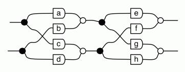
corresponds to the matrix $\left(\begin{array}{cc} a & b \\ c & d\end{array}\right)$ . In general, the number of columns of the corresponding matrix is the number of dangling wires on the left, and the number of rows is the number of dangling wires on the right. Moreover, the entry at row i and column j is the number of paths from the jth wire on the left to the ith wire on the right.

Finally, the composition

corresponds to the matrix obtained by performing the matrix multiplication ①.

And, as you’ve seen, it all follows from how adding and copying interact!

Continue reading with Episode 11 – From Diagrams to Matrices

Graphical Linear Algebra

Menu

Category Archives: Matrices