18. Introducing the Antipode

I was in Nijmegen all of last week, attending the CALCO and MFPS conferences.

On the plus side, they were both excellent and featured many really nice talks. Being bombarded by so much new research always gives you a whole load of ideas. And apart from the scheduled talks, the coffee breaks and the evening events give you a chance to discuss with a large number of extremely interesting people. All of this takes its toll: after an intensive conference week you really get the urge to lie down and sleep for 20 hours so that your brain can get the chance to organise all the new information!

So, on the minus side, the sheer number of talks and social events meant that I have had no time to work on this blog. Overall, it’s going to be a really busy summer for me, so the frequency of articles will drop a bit. Maybe it’s for the best, I’ve been told by a number of people that it’s been difficult to keep up.

I presented my paper with Apiwat Chantawibul on using string diagrams as a language for graph theory at MFPS. I had some really nice questions and I found out from Nicolas Guenot that very similar diagrams are used in something called deep inference in logic. I have to investigate this, it looks extremely interesting! Surely it cannot be a coincidence that their diagrams are so similar. Eventually I’ll have write about that research thread on this blog.

The history of mathematics is delineated by a number of events where, in order to make progress, new kinds of numbers were introduced. These impostor-numbers were usually first used as a technical trick to “make the calculations go through”. Then, after a while, they began to be taken a bit more seriously, before being finally dismissed as “totally obvious” and taught to primary school kids. Zero is a prime example, and it was surely very controversial, although we have lost a great deal of the debates because they happened so long ago. Negative numbers are another example. First discovered in China around 200 BC, they were routinely degraded as confusing, unnatural and generally nefarious until the 19th (!) century. Fractions, aka the rational numbers are yet another instance of this phenomenon, and we will discuss them here in a few episodes. More recently the story has been repeated for other kinds of numbers, the complex numbers being probably the most famous. But we have to wait until the final years of high school before meeting them, and we still refer to some of them as imaginary.

To make progress in graphical linear algebra we need to add negative numbers to the diagrammatic language. Back in Episo de 7 I told you that graphical linear algebra has five principal actors. We have met four of them so far: copy and add, together with their sidekicks discard and zero. We meet the fifth one today. The new actor—being a trickster— likes to impersonate the natural numbers, so let’s first remind ourselves of what the natural numbers are, diagrammatically speaking.

We have discovered that the natural numbers can be identified with those diagrams in the system B that have precisely one dangling wire on the left and one on the right. This was done in two steps: first we introduced the syntactic sugar for natural numbers in Episode 9, and then in Episode 16 we argued that every diagram of this kind (one dangling wire on each end) is equal to one that arises from a sugar. This fact is a consequence of the more general faithfulness theorem for the homomorphism of PROPs θ from B to the PROP Mat of natural number matrices.

Let’s remind ourselves of the properties satisfied by these diagrams. All of the following are theorems, which we proved using only the basic equations that capture how the copying generators interact with the adding generators.

Our fifth principal actor is called the Antipode—Minus One to its friends. The antipode generator is a flamboyant character. It’s a bit of a rebel, in that it looks quite a bit different to the other characters we have met so far. This is how it will appear in this blog:

First, the colour: it’s red. This is motivated by the fact that we want the bizarro of antipode to be itself, just like the bizarro of every natural number is itself. If we coloured the antipode black or white, then this would be incompatible with our convention that bizarro, syntactically speaking, means reflecting and swapping black with white. We thus exclude red from the colour swapping game. In any case, red seems like a good choice for negative quantities: after all, if you have negative money, then you are said to be “in the red“.

Second, the shape: it’s square. This contrasts with the shape of the sugars for natural numbers and matrices, which we have been pointing to the right, corresponding to the direction that numbers travel along the wires in our circuits. The fact that the antipode doesn’t play by the same rules is not an arbitrary choice, as we will see in a few episodes.

Let’s get an idea for what the antipode does, using the intuition of numbers travelling along wires. As we have seen in Episode 9, the natural number sugars act by multiplying their input by the natural number they represent. Similarly, the antipode acts by multiplying its input by -1. So, if a number x arrives on the left dangling wire, the number -x will exit on the right dangling wire, like so:

It’s time to meet the equations that involve the antipode. The antipode pretends to be a number; but unlike natural numbers it is a bona fide generator and not defined in terms of other generators. We therefore need to take some of the properties satisfied by natural numbers as basic equations of the expanded system.

Let’s start with how the antipode relates to the copying structure. First we have the antipode version of (copying):

that says that multiplying any number by -1 and then copying it gives the same results as if we had first copied the number and then multiplied each copy by -1. Next we have an equation that resembles (discarding):

which simply says that multiplying any number by -1 and discarding it is the same as simply discarding.

The bizarro versions of (A2) and (A3) are included as well. The first of these is the following, which is the antipode equation that corresponds to (adding).

It can be understood as saying that for all numbers x and y we have that -(x + y) = -x + -y. Finally, we have the fact that -0 = 0, which is the antipode version of (zero).

Clearly, in each of (A2), (A3), (A4) and (A5) the behaviour of the left hand side and the right hand side is the same.

The final and most important equation tells us how that antipode acts as the additive inverse of 1. Interestingly, it is the only equation of the system that involves all the generators that we have seen so far!

Since it is the most important, let’s spend a little bit of time understanding why it is compatible with our intuitions. First the left hand side.

A number x arrives on the left, it is copied and the first copy passes through the antipode. So -x and x are fed to the adder, which then spits out -x+x.

The right hand side of (A1) accepts x on the left and emits 0 on the right. But for any x we have that -x+x=0, so the behaviours of the two sides agree.

That takes care of all the equations we need. Let’s collect the entire expanded system in a handy cheat sheet:

We gave the name B to the diagrammatic language described by the first three panels, which stands for (bicommutative) bimonoids, or bialgebras. We will refer to the expanded system that includes the antipode generator and equations (A1)–(A5) as H, which stands for (bicommutative) Hopf monoids or Hopf algebras, which is the name that these structures are often called by mathematicians.

There are a number of interesting things that we can prove, using the basic equations. The first is that composing the antipode with itself gives the identity wire, which is the diagrammatic way of saying that -1⋅-1 = 1.

Another useful fact is that the antipode commutes with all the other natural numbers. That is, for all natural numbers n, we have the following:

We can prove this property by induction. First, the case n=0:

and the inductive step, for n=k+1:

We will now extend the syntactic sugar for natural numbers to integers; indeed, the antipode gives us a nice way to consider all integers diagrammatically. Since we already know how to deal with zero and the positive integers, the only remaining case is negative integers. Here, assuming that n is a positive natural number, we can define:

This extension of the syntactic sugar from natural numbers to integers seems to be simple enough, but how do we know that it “really works”? One way of making sure is to check that the algebra of integers as we know it is compatible with the algebra of diagrams: properties such as (multiplication) and (sum) ought to work for all the integers.

So, let’s assume from now on that u and v are (possibly negative) integers. First, let’s consider the multiplication property:

This is easy to prove from the facts that we have already established: the antipode commutes with the natural numbers and, diagrammatically, -1 ⋅ -1 = 1. Since we already know from Episode 9 that (multiplication) holds when u and v are positive, it’s enough to consider the cases where one or both of them are negative. Try it yourself!

To prove that summing up two integers works as expected takes a little bit more work. We want to prove the following:

When u and v are both non-negative then we do not have to do anything; we already proved this property by induction in Episode 9. If u and v are both negative then they are of the form -m and -n for some positive m and n. So let’s show that the property holds in that case:

In the first and the last line we used the definition of the sugar for negative integers, and in the second last line the property (sum) for natural numbers. And, of course, -(m+n)=(-m)+(-n), so we’re done.

We are left with the case where precisely one of u and v is positive and the other negative. Without loss of generality, we can assume that u is negative, that is, it is of the form -m where m is a natural number, and v is non-negative, that is, it is a natural number n. We don’t lose generality because if they were in the other order, we could simply swap them using commutativity of sum, which we proved in the last episode.

The idea now is to do a simultaneous induction on m and n. The base cases, where m or n (or both) are 0, are simple to verify: try it. Once we have established the base cases, the inductive case goes as follows:

In the third and the fourth line of the proof above we used the definition and a useful property of the syntactic sugar from Episode 10. The final thing to notice is that -(k + 1) + ( l + 1) = -k + -1 + l + 1 = -k + l + -1 + 1 = -k + l. That completes the proof of the claim that (sum) works for all integers.

The final thing to be said is that also (copying), (discarding), (adding) and (zero) hold for all integers: this is easy to see since they hold for natural numbers and equations (A2)–(A5) postulate that they hold for the antipode generator. Armed with this knowledge we can prove, for example, that multiplication distributes over addition for integers.

In the next episode we will see that just as the diagrammatic system B gave us a diagrammatic language for matrices of natural numbers, system H gives us a language for matrices of integers. Then we will be able to move on to the really cool stuff!

Continue reading with Episode 19 – Integer Matrices.

17. Maths with Diagrams

The discussion over the last few episodes has now led us to the point where we have two different languages to talk about the same thing. The two languages, however, are rather different. One consists of diagrams, the other of matrices populated with natural numbers. If you already knew about matrix algebra, maybe you’re asking yourself the question “What’s the point of all these diagrams then? They don’t tell me anything that I didn’t know before. Is this guy claiming that this diagrammatic language is better in some way?”

The short answer is no. I don’t want anyone to throw away their matrices: there are extremely good reasons to know and care about them. But I have two arguments for why we should also care about diagrams.

The first argument is that a different language means thinking about the conceptual landscape in a new way. We will see this over and over again in graphical linear algebra, and sometimes it will cause us to reevaluate certain dogmas: ways of doing things that have come about because of the way that the standard notation works, rather than real underlying mathematical issues. These kind of things are not easy to spot if you only know one notation.

More generally, the idea that the languages we use influence how we think and act—linguistic relativity if you will—is well-known and appreciated by programmers. Most programming languages are Turing complete and so have equivalent power. So why not just learn one, say x86 assembly, and stick with it?

Programmers deal with real problems, which usually do not involve writing functions to compute the Fibonacci sequence or, infamously, inverting a binary tree. Real problems are multi-faceted, and for some parts it may be useful to put on a functional hat, for others an object-oriented hat, and so on. The different ways of thinking that the various programming methodologies bring to the table are appreciated because

complex problems benefit from a combination of approaches.

When I was a student in the 90s that there were many entertaining flame-wars about which programming language approach was the best. As with most flame-wars, they were pretty pointless: programming has since grown up and nowadays it’s very rare to hear somebody claiming that a particular way of doing things is intrinsically better than another. Good programmers are comfortable thinking in several different languages, and choose the one that is most suitable for the current (sub)problem at hand. Flexibility is key.

Because of this, in the last 10 years or so, the boundaries between different language families have been blurring. For example, most functional programming languages have clever ways to do imperative things, and conversely, more and more functional features are making their way into industrial strength imperative languages. It’s pointless to argue which is the best approach, or the best language: such a thing doesn’t and will never exist. And anyway, it’s fun to see how your favourite problems can be solved with some newfangled language!

It’s been really interesting to see how different communities have reacted to this blog. About a month ago somebody posted a link to this blog on Hacker News. That link made it to the front page and resulted in a massive amount of interest, which really surprised me… who knew that so many people cared about linear algebra! Last week I posted a link there myself and again the feedback has been really great. I’ve also been regularly posting links on Reddit’s /r/math, which has also resulted in a lot of really interesting and useful comments, but also quite a bit of skepticism and maybe even a touch of hostility.

Allow me to philosophise for a moment for why this is the case. I think that it’s because many mathematicians are just not used to the idea of having different languages to talk about their concepts. In many mathematical subfields the notation is very conservative and standardised. It has evolved so slowly, so imperceptibly, that mathematical culture almost brings with an an understanding that “standard notation” has been given to us by some higher power and it is not to be disturbed. Anyway, the concepts are the important things so who cares about notation. Many mathematicians simply don’t see the value in exploring different ways of expressing themselves. Programmers, it seems, are much more receptive to the idea.

The second argument for why we should care about diagrams is Occam’s razor — the idea that one should trim the fat: discard unnecessary assumptions to try to get at the core of problems. So let’s consider the amount of intellectual technology necessary to develop the concept of

matrices of natural numbers, and their algebra ①

I need you to forget for one moment that you know all of these things already and that they are totally obvious to you; let’s pretend, for one moment, that we are explaining Earth mathematics to a group of interested Martians. And let’s not be too creative about the Martians. Let’s assume that they are of the Star Trek variety: three dimensional and humanoid enough to interest Dr McCoy in extra-curricular activities, but without the experience of an Earth education. So, to make them understand what ① means, we need to:

Explain the concept of natural numbers, together with addition and multiplication
Show that the natural numbers form what is called a commutative semiring. Let’s go through these requirements:
1. addition is associative, commutative, and has 0 as it’s identity; that is, for any natural number n, we have 0 + n = n = n + 0
2. multiplication is associative, commutative and has 1 as it’s identity; that is, for any natural number n, we have 1· n = n = n · 1
3. multiplication distributes over addition, that is, for all natural numbers a,b and c, we have a·(b + c) = a·b + a·c (in a non-commutative semiring we would also require (b+c)·a = b·a + c·a, but that follows here from commutativity of multiplication)
Define the concept of an m×n matrix, a grid of numbers. If we are totally honest then we ought to probably also go through the corner cases where any combination of m and n can be 0.
Write down the formula for matrix multiplication. This relies on already knowing about addition and multiplication of natural numbers. The semiring properties are necessary for matrix multiplication to behave as expected (e.g. for it to be associative).
Write down the formula for matrix addition.

This is actually a significant amount of work. And maybe the Martians are a bit curious about where exactly did the formula for multiplying matrices came from. They know from previous Earth experience that you can’t really trust those pesky humans and their crazy ideas.

On the other hand, we have already done all of the work of showing how diagrams work in the first few episodes of this blog. If explaining to the Martians, we would need to:

Explain the idea of magic Lego; the algebra of diagrams that consists of the two operations of direct sum ⊕ and composition ;
Go through the rules of diagrammatic reasoning: stretching, tightening, moving generators along wires
Introduce the four generators together with the ten equations.

Let’s compare the two ways. In the traditional approach, one first defines the natural numbers and then “bootstraps” matrices on top. With diagrams, there is no precedence given to natural numbers as such; everything gets defined at the same time. Natural numbers can be recovered as special kinds of diagrams, those with one dangling wire on each end. We don’t need to invent any extra formulas for multiplying matrices because composition is a basic operation of the algebra of diagrams. Matrix addition is not a primitive operation at all, it can be constructed from the diagrammatic primitives.

Having said all that, this blog so far has followed a rather conventional route: first we talked of natural numbers as diagrams and then of matrices as diagrams. Today, we are going to go back and think about how the maths would have been developed without knowing about natural numbers and matrices from the outset. We will rediscover diagrams by focussing on the operations and constructions that are natural in their language and see where that takes us.

To spice things up let’s try some alternate history. This is something that historians really hate; my sister, who is a historian, always gets annoyed when I bring it up. But who doesn’t love to annoy their siblings?

We need to turn the clock back to before matrices were common, before notation settled into what appears in textbooks today. Our story thus takes place in early 13th century Pisa. Our hero is a certain young man, Fibonchi, a contemporary and friend of Fibonacci.

While a teenager, Fibonchi sailed to the Balearic Islands with a Pisan trade fleet. In Palma, he met a wise old Berber merchant who introduced him to four curious operations that spoke of putting things together and copying them, governed by collection of simple, self-evident rules. The old men of Palma enjoyed drawing the diagrams and even used them to perform some calculations.

On his way back home, Fibonchi realised that the diagrams are what is now known as a recursive data type: every diagram is put together from the four simple bricks, the identity and twist. Using this insight, he was able to prove a number of interesting things about them, using the principle of induction.

To help in his calculations Fibonchi wrote down the formula for diagrams that copy and add not just one wire, but an arbitrary number on wires. Coincidentally, this was the syntactic sugar we discussed a couple of episodes back.

Next, Fibonchi proved that these sugars satisfied a very pleasing property with respect to arbitrary diagrams. For example, given any diagram D with m dangling wires on the left and n dangling wires on the right, the following is true:

Of course, once Fibonchi had finished this proof, he immediately wrote down his second theorem.

He did not even bother writing down a proof, since he was told about about the principle of “bizarro” by the old man in Palma. Because all the equations in the system have bizarro (reflected, colour-swapped) versions, once you proved a theorem you’ve also proved its bizarro cousin.

Fibonchi also noticed the following two related facts, the second the bizarro version of the first.

These properties intrigued Fibonchi, and he went ahead and defined an operation on compatible diagrams—those that agreed in their respective numbers of dangling wires on the left and right. He called the operation sum. This operation would be rediscovered in different notation a few centuries later and given the name matrix addition.

He proved that sum was associative

and commutative:

Moreover, each compatible family of diagrams contained an identity for this operation:

Fibonchi showed that D + 0_m,n = D = 0_m,n + D.

He also noticed that composition distributes over sum: we have

D ; (E+F) = D ; E + D ; F

The proof, reproduced below, was a straightforward application of his first theorem.

He was, of course, immediately able to state the bizarro version:

(D+E) ; F = (D ; F) + (E ; F)

Fibonchi knew that composition of diagrams was not commutative, in most examples it didn’t even make sense to compose diagrams in more than one way because the dangling wires did not match up. Non-commutativity was the norm. However, he did notice some peculiar things about diagrams with exactly one dangling wire on each end.

He noted that there was exactly one such diagram for every natural number, which gives the number of paths from the left dangling point to the right one. He understood that if two such diagrams have an equal number of paths then they are equal. His arguments were close to the rewriting argument of the last episode. Another strange thing was that the bizarro of every such diagram was equal to the diagram you started with.

Most curiously of all, composition between such diagrams was commutative, which Fibonchi confirmed with a simple induction. First the base case, where the first diagram has zero paths:

and the inductive step:

Inspired by Fibonacci’s masterpiece Liber Abaci, Fibonchi wrote his own treatise entitled Liber Diagrammatis. Unfortunately it is now lost; the last remaining copy fell into the hands of a Livornese fishmonger sometime in late 16th century, who used it to wrap his wares. The Livornese never much liked the Pisans or what they had to say.

Fortunately, we can continue Fibonchi’s story on this blog.

Continue reading with Episode 18 – Introducing the Antipode.

16. Trust the Homomorphism, for it is Fully Faithful

Last time we proved that θ—the homomorphism that takes diagrams to matrices—is full. This means, roughly speaking, that for any matrix there is at least one corresponding diagram. Moreover, starting with an arbitrary matrix, we actually gave a recipe to construct a diagram that does the job. This provides us with a useful syntactic sugar, since any m×n matrix of natural numbers can now be considered as a diagram with n dangling wires on the left and m on the right. The construction extended the sugar for natural numbers from Episode 9.

There is still one final, thorny issue regarding θ that we ought to be nervous about. What if there are more diagrams than matrices? Or, more precisely, can we identify two different diagrams that go, via θ, to the same matrix? Then θ would not be perfect for the same reasons that “serendipity” and “dog” should not translate to the same word in French.

This final fear is laid to rest today as we tackle faithfulness. Once we know that θ is both full and faithful (or “fully faithful”) we can finally conclude that θ is a perfect translation; an isomorphism of PROPs.

The proof that θ is faithful is a little bit tricky. Let’s start by reminding ourselves of what faithfulness means: whenever two diagrams D₁ and D₂ are different, then the matrices θD₁ and θD₂ must also be different:

D₁ ≠ D₂ implies θD₁ ≠ θD₂ ①

This is logically equivalent to saying that, for any diagrams D₁and D₂, if θD₁ happens to be equal to θD₂ then D₁ and D₂must have been equal to begin with.

θD₁= θD₂ implies D₁= D₂ ②

In spite of the logical equivalence of ① and ②, the formulation in ② is somewhat easier to turn into a proof. So let’s focus on what ② is saying. Given a diagram D, θD is table of numbers that record the numbers of paths from each dangling point on the left to each dangling point on the right in D. Then, to prove ②, we need to find a way of showing that:

whenever two diagrams have the same numbers of paths then they are equal.

And we consider two diagrams equal exactly when we can find a diagrammatic proof of this fact, using a combination of diagrammatic reasoning and our ten equations, repeated below.

We will outline two different ways to prove faithfulness. They both concern the four equations (B1)-(B4) that tell us what happens when adding meets copying. As we will see, the two different techniques each have their strengths and weaknesses, and for that reason it’s useful to have both in our toolbox.

The story naturally begins with diagrams that have a very particular shape: all of the copying comes before all of the adding. Let’s be a bit more precise: we mean those diagrams in which we can find a point to draw a vertical separator, so that the following condition is satisfied: the only generators allowed to the left of the separator are the black ones (copy and discard); and to the right of it the white ones (add and zero). Here’s a picture:

and here’s an example of a diagram in this form.

To the left of the separator we have two copy generators, and to the right we have two addition generators and a twist. The twist is allowed on either side of the separator: this is because in our discussion about PROPs we understood that the twist is not a generator, even if we do consider it a basic brick of our diagrammatic language. The twist, aka σ_1,1, is a part of the permutation structure expected in any PROP. In particular, another way of positioning the separator is the following, where the twist is now to the left of the separator.

Here’s a simple non-example for comparison: we cannot find a place to put in a separator, because the addition comes before the copying.

Moreover, because the addition generator connects directly to the copy generator, we cannot use any of our vanilla diagrammatic reasoning, such as sliding along wires. We could, however, use the (B1) equation in our system to replace this diagram with the previous one, which has the right shape.

Most of the work of proving faithfulness is showing that every diagram can be transformed using our equations and diagrammatic reasoning into one in which the copying and the adding can be separated. This is because such diagrams are almost matrices, as we will now see.

Here’s what we mean by this rather cryptic remark: using the syntactic sugar for copy and add from Episode 10 together with the syntactic sugar for natural numbers from Episode 9, we can easily transform any such diagram into matrix form. Diagrams in matrix form look like this:

It’s easy to see that the matrix that results from applying θ to the diagram above is none other than:

So the entries can be read directly off the diagram: we simply scan down the centre to fill out the matrix.

Let’s go through an example to see how this works: it is not difficult to generalise the procedure to any diagram where the copying comes before the adding. Consider the diagram below. It is of the right shape, because we can draw a separator that walls off the black structure from the white structure.
We start by cleaning the diagram up a little bit. We can use (Unit) and (Counit) to make some redundant zeros and discards disappear, and use diagrammatic reasoning to move the ones that remain so that they are right next to the boundary and don’t cause any further problems. In our example, this means using (Counit) to get rid of the discard at the bottom left, and pulling in the zero over on the right. We end up with the diagram below.

Next we introduce the syntactic sugar for copying and adding that gets rid of chains of copies and adds. In our example this means the following:

Next we clean up even more: we eat up any annoying permutations (like the one at the bottom right) with the sugars, and collect compatible paths—those with the same dangling points—using our natural number sugar.

We could really stop here, but being the pedantic sticklers that we are, we can slide the numbers along, and add 1s and 0s to get the diagram looking exactly like the template.

But why bother to go to all this trouble?

The reason is that once we have a diagram D in matrix form, the relationship with its matrix θD is extremely tight since we can read off each matrix entry just by scanning down the middle of the diagram. This close connection can be exploited to prove faithfulness: when D₁ and D₂ are in matrix form, and θD₁ is the same matrix as θD₂, they clearly must be equal as diagrams!

So, in general, the question of faithfulness boils down to the following:

Can we transform any diagram into matrix form?

And, since we have just argued that any matrix in which copying comes before adding can be put into matrix form, the central question to consider becomes even simpler:

Can we transform any diagram so that copying comes before adding?

By the way, we have been putting diagrams in matrix form already without realising it. In Episode 10, we showed how go from the diagram on the left below—which totally fails to be in matrix form since some add generators come before copy generators—to the diagram on the right, which is in matrix form. The procedure of putting a diagram in matrix form is thus closely connected with the concept of matrix multiplication.

It’s time to discuss one of the ways that we can answer the question. Putting the copying before the adding means focussing on what happens when the two structures interact. That story is captured by our four equations.

When we first discussed them in Episode 8, I mentioned that these equations amount to something called a distributive law of PROPs.

We will not go through the details of what this means now, but the upshot is that any diagram D can be factorised (a more fancy way of saying “transformed into a form in which we can find a suitable point to put in a separator”) so that D = C ; A, where C is a diagram that uses only the copy and discard generators, and A only the add and zero generators. So the work comes down to showing that the rules (B1)-(B4) actually amount to a distributive law. Fortunately, Steve Lack considers this very example in Composing PROPs, it is Example 5.3 in that paper. The deeper story behind all this is actually both extremely interesting and enlightening, but it requires a little bit more category theory. We will come back to it eventually.

Overall, the strength of using this technique is that… we didn’t really have to do very much. For austere, beautiful mathematical reasons, the equations give us a distributive law and guarantee that that the factorisations we need always exist. But if you give me a diagram and tell me to find an actual factorisation then I don’t have very much to go on: I know it exists, but the distributive law does not tell me how to find it. Nevertheless, it is enough to prove faithfulness, so we should not complain too much.

The second way of showing that every diagram can be factorised relies on a technique called rewriting. The basic idea is that, instead of considering (B1)-(B4) as equations, we orient them and consider them as rules.

Then, the strategy is to find left hand side of one of the rules in our diagram. This is called a match for that rule, and if we can find it, we replace it with the rule’s right hand side. Next, we keep repeating these two steps until we there are no more matches. The rules take care of all the possible ways that white structure can come before black structure, so if we cannot find any matches then we have essentially found the factorisation.

Sounds simple enough, but there are a few complications. Let’s go through an example to get a feel for what’s going on. Our starting diagram is drawn below, and already we have found a match for one of the rules; it’s the area highlighted within the red rectangle.

So we replace the match with the right hand side of the rule, obtaining the diagram below.

The red box in the second diagram is highlighting another match, which we can then replace with a right hand side of the relevant rule. Let’s keep repeating this procedure to see where we end up.

Now we seem to be almost finished, but there’s still an add connected to a discard, highlighted in the last diagram above. We do have a rule for that, but the match is complicated by the fact that there is a twist in the middle. So, if we were going to implement this in software, we’d have to make sure that our algorithm for finding matches takes these kinds of situations into account. And after this final step the diagram becomes

where there are no more bad connections. We can now simply use diagrammatic reasoning to pull all of the black structure to the left and the white structure to the right, obtaining a factorisation.

Another, more radical, way to deal with the issue of matches is to go back to the drawing board and change the way we think about diagrams. We have been thinking of diagrams as magic Lego, built up of basic tiles that connect to other basic tiles. But we could start thinking of them as graphs with white nodes and black nodes. Then, the rewriting we have been discussing becomes a kind of graph rewriting.

This is the approach taken by Aleks Kissinger at Oxford, who has developed the Quantomatic software package for working with string diagrams. Aleks and his collaborators have developed a whole load of really cool new technology, and I hope to convince him to eventually write a few articles on this blog, explaining some of the latest developments!

There is one more issue to consider when dealing with rewriting: termination. Let’s look at the first step of our rewriting example again. In the first diagram, there is only one match. But by applying the rewrite rule, we ended up in a diagram with three different matches. It seems that we’ve cut of the head of the Hydra only for three heads to pop up again. If this kind of thing continues indefinitely, then as much as we rewrite, we will never finish.

This thing about rewriting systems in general, is that:

they may look simple and intuitive
but it is often surprisingly tough to prove that they terminate.

Fortunately, the rewriting system above does terminate. We will prove it eventually on this blog, but you’re welcome to try it yourself; it’s not so trivial!

There are several people studying rewriting theory on diagrams like ours. For example, Samuel Mimram at the École Polytechnique has recently been doing some very exciting work on techniques that simplify the process of proving properties like termination.

Summing up: if we use the distributive law then we don’t have to work very hard but we don’t get a factorisation algorithm. If we use rewriting then we have an algorithm but we have to work quite hard to prove that it works. Such is life.

This episode concludes the work of showing that θ is an isomorphism. We have spent quite a bit of time discussing the mathematics of diagrams. This was all very useful because, after all the hard work, we now have a much firmer handle on how to work with them. But, as interesting as it is, the mathematics of diagrams is not really the main point of this blog, which is doing mathematics with diagrams. This is the subject of the next episode.

Continue reading with Episode 17 – Maths with Diagrams

15. Matrices, diagrammatically

We have established that there is a homomorphism called θ from B, the PROP of diagrams, to Mat, the PROP of matrices. To do this, it was enough to say where θ takes the four stars of the story so far: the add, zero, copy and discard generators.

The task for this and the next episode is to understand why θ is an isomorphism—a perfect translation—and to show that a PROP homomorphism is an isomorphism, it is enough to show that it is full and faithful.

The intuition for why the translation works well was established all the way back in Episode 10. The idea is that a diagram with n dangling wires on the left and m on the right translates to a matrix with n columns and m rows. In that matrix, the entry in the ith row and the jth column of the matrix is the number of paths from the jth dangling point on the left to the ith dangling point on the right in the diagram. It’s not difficult to verify that this is exactly how θ works: for example we have the following:

Now, to show that θ is full, we just need to convince ourselves that every matrix has a diagram that translates to it.

In fact, this may already seem to be pretty straightforward, given what we know about paths. If I give you some matrix then—looking at the example above for guidance—you should be able to go away and draw a diagram that does the job. Still, intuition doesn’t always cut the mustard, so it’s worthwhile to spend some time doing this properly. That’s our task for today. The proof of fullness also provides us with new syntactic sugars that make the diagrammatic language even nicer to use.

In Episode 9 we saw how diagrams with one wire dangling on the left and one on the right can be identified with the natural numbers. By now we know a whole lot more about diagrams. Today we will see that the diagram for a natural number n translates via θ to the 1×1 matrix (n). The proof that θ is full is the continuation of this story, since it amounts to building up a diagram for any matrix of any size.

Before we launch into the proof, we need to introduce a new family of syntactic sugars, one for each natural number m. Their names are m-copy and m-addition, and, just like copy and add, one is the bizarro version of the other. We therefore only need to concentrate on thinking about one, since the story for the other is simply the bizarro version.

Our old friend, the copy generator, has a single dangling wire on the left, and our standard intuition says that it works by copying whatever value appears on that wire to its two wires on the right. But what if there are values arriving on two or more wires, and we want to copy all of them? For example, in the case of two wires we would need to construct a circuit that has two dangling wires on the left and four on the right that behaves as follows, for any numbers x and y:

We can wire up an such a diagram using two copy constructors and a twist: we copy the x and the y, obtaining two xs and two ys, then we swap an x and y. Like this:

It seems that it should be fairly straightforward to construct such a gadget for three wires, four wires, and so on, using only copy, identity and twist. This is the idea of m-copy, where m is a positive integer, and we will draw it like this:

The white m in the middle of the black circle refers to the number of wires being copied. The black ms on the wires are a sugar that we have already seen: they mean m stacked identity wires, or m-wires for short.

The picture of the sugar is a bit busy with all of those ms. We want to keep our diagrams looking sharp, so when we use m-copies we will typically be a bit lax with writing all of these numbers. Just keep in mind that whenever you see one, it has an m-wire dangling on the left, and two m-wires dangling on the right. One more thing: if you want to draw this sugar on paper and you don’t have access to white pens, feel free to write the number above the circle.

Let’s go ahead and define it, using recursion. The base case, m = 1, is just the copy generator.

Next, the recursive case is:

So, to copy k + 1 wires, we can copy the first k wires recursively, copy the last wire, and then we have to make sure that the dangling wires line up properly on the right, using σ_k,1. We have already seen the case m = 2, so here’s what the construction gives us for m = 3:If, unlike me, you have a good memory, you probably remember a different sugar for copy, which we introduced in Episode 10. There we chained several copies one after the other, obtaining a copy sugar that has one dangling wire on the left and several on the right. Both the sugars are useful, and it’s possible to use them together, but it is important not confuse them.

It’s interesting to think about the matrices that correspond to m-copy. So let’s take a look at the first two:

The pattern is becoming apparent: in general, it’s not difficult to show that for an m-copy, the corresponding matrix is formed by stacking two identity matrices of size m, as illustrated below.

Although we don’t strictly need this for our fullness proof, in the future it will be useful to know that m-copy satisfies the same kind of equations as ordinary (1-)copy. In particular, there is the m-version of (CoComm):

where the role of the twist is played by σ_m,m. The proof is a pretty straightforward induction, and we will skip it. Similarly, we can prove an m-version of (CoAssoc)

and an m-version of (CoUnit).

The left hand side of the last equation features a new, but very simple, sugar: the m-discard: this is simply m discard generators stacked on top of each other. For example, this last equation, when instantiated at m = 2, looks like this when de-sugared:

The bizarro version of the m-copy sugar will also come in handy for us. Just as addition is the bizarro copy, m-addition is the bizarro m-copy. Being bizarro, we do not need to define it from scratch since we can take the recursive definition of m-copy, reflect it and invert the colours. But let’s just understand what it means in terms of our intuition; for example, the behaviour of 2-addition is as follows.

Following our bizarro tradition, we will draw m-addition like this:

and, just as expected, m-addition satisfies the m-versions of the adding equations.

These are:

The last equation features m-zero, which similarly to the m-discard, is simply m zero generators direct summed together.

Finally, let’s think about the matrices that correspond to m-addition. We already know that bizarro in the matrix world means transpose matrix, so it’s not surprising that we have:

We are ready to prove that θ is full, that is, given any m×n matrix A, there exists a diagram D such that θD = A. Let’s first consider the corner cases: m = 0, n = 0 or both m = n = 0.

When m = n = 0, there is precisely one matrix with 0 columns and 0 rows, the empty matrix (): 0 → 0. Coincidently, there is a diagram with 0 dangling wires on both ends, the empty diagram. Both the matrix and the diagram are actually id₀ in their corresponding PROPs, so θ by definition takes the empty diagram to the empty matrix.

When n = 0, m ≠ 0, the diagram that does the job is the m-zero. Similarly, when n ≠ 0, m = 0, the diagram that does the job is the n-discard.

The interesting part of the proof concerns m×n matrices where m,n≥1. Our proof is divided into three parts, and each part is an induction. In Part 1 we will handle 1×1 matrices, next the column vectors (m×1 matrices) in Part 2, and finally in Part 3 matrices of arbitrary size (m×n). Each part uses the results of the previous parts.

Part 1

Let’s get started by showing that fullness holds for every 1×1 matrix. What we want to prove is that, for any natural number a, we have:

where the diagram in the left hand side is the our diagrammatic sugar for natural numbers, which was the topic of Episode 9.

We can prove it by induction on a, the base case is:

where, by definition of composition in the PROP Mat of matrices, we multiply the unique 1×0 matrix with the unique 0x1 matrix. The result is a 1×1 matrix, and following the formula for matrix multiplication, it is the empty sum. And the number you get after adding up zero things is zero. So far so good.

Now for the inductive step: let’s assume that the claim holds for a = k, and show it for a = k + 1.

In the first step we use the recursive definition of the natural number sugar, and in the next two steps we use the definition of θ. We use the the inductive hypothesis in the fourth step. Next we just perform the calculation in the PROP of matrices. That completes the job for 1×1 matrices.

Part 2

Using what we already know, we will show that every column vector, that is, every m×1 matrix has a diagram that maps to it via θ. Again we do it using induction, but this time on the height of the vector, m. The base case is 1×1 matrices, which we have established in Part 1.

So, let’s do the inductive step: supposing that fullness holds for k×1 matrices, we want to show that it holds for (k + 1)×1 matrices. The key observation here is that every such matrix looks like this:

where v is a column vector of height k and a is some natural number. Using the inductive hypothesis, we know that there exists some diagram (that we may as well call v) with one dangling wire on the left and k on the right, such that:

Using this inductive hypothesis and our result from Part 1, we can build a diagram for the larger column vector:

and this completes the job. So we now know how to construct diagrams for column vectors of arbitrary size.

Part 3

This final part concentrates on arbitrary m×n matrices. The induction, this time, is on n. The base case is m×1 matrices, and we found out how to deal with these in Part 2.

Now, assuming that we can construct diagrams for m×k matrices, we need to show that we can construct them for m × (k + 1) matrices. The observation that we can make here is that any such matrix looks like this:

where A is some m×k matrix and v is a column vector tacked on at the end. The inductive hypothesis tells us that we have a diagram that translates to A:

and we can use this to construct a diagram for the larger matrix. To do this, we make use of the m-addition sugar that we cooked up before and the fact, shown in Part 2, that we know how to get a diagram for v.

That completes the proof: θ is full, as advertised.

Back in Episode 9 we introduced a syntactic sugar for natural numbers as certain diagrams. The proof of fullness shows us how to extend this to a sugar for any m×n matrix.

This means, that given a m×n matrix A, we have a diagram

We can reinterpret the induction proof, working back from Part 3 to Part 2, to obtain a recursive definition for this sugar, extending the natural number sugar of Episode 9:

This sugar will be quite useful for us as we do more graphical linear algebra, since it will allow us to consider any matrix of natural numbers as a diagram!

Continue reading with Episode 16 – Trust the Homomorphism, for it is Fully Faithful

14. Homomorphisms of PROPs

In the last two episodes we have established that our diagrams, constructed from the four generators, and subject to the equations below, are the arrows of a PROP B.

We have also talked about another PROP, Mat, that has as its arrows matrices of natural numbers.

In maths, it is often the case that to understand something properly you need to think about how it relates to other things. Our current task is an example of this, since we need to establish exactly what we mean when we say that diagrams and matrices “are the same thing”. This brings us to the notion of homomorphism —a generic jargon word that means “structure-preserving translation”—of PROPs.

So suppose that X and Y are PROPs. It’s useful to colour them so that we can keep track of what’s going on in which world, the red world of X and the hot pink world of Y. A homomorphism F from X to Y (written F : X → Y) is a function (a translation) that

for any arrow A : m → n in X produces an arrow FA : m → n in Y.

Notice that the domain and the codomain must be preserved by the translation: both A in X and FA in Y have domain m and codomain n.

But PROPs come with a lot of structure, and homomorphisms have to preserve all of it. For example, for any other arrow A’ in X, it must be the case that

F(A ⊕ A’) = FA ⊕ FA’ ①

The above equation says that if I translate the monoidal product of A and A’ taken in X then I get the same thing as if I had translated A and A’ separately and took the monoidal product in Y. Remember that monoidal product is defined differently in different PROPs: for example in B it is the stacking diagrams on top of each other, while in Mat it is forming a certain matrix.

Similarly, if we can compose A with A’ (which we can do exactly when the domain of A’ is n) then:

F(A ; A’) = FA ; FA’ ②

Again this says that translating A composed with A’ in X should be the same thing as translating the individual components separately and doing the composition in Y. Recall that in B composition is simply connecting dangling wires together, while in Mat it is matrix multiplication.

Moreover, as we have seen, every PROP has special identity arrows, one for each natural number m. These form a part of the structure of PROPs and so must also be preserved:

Fid_m = id_m ③

Finally, for any natural numbers m, n, there are the special “wire-crossing” arrows σ_m,n that also must be preserved:

Fσ_m,n = σ_m,n ④

That takes care of all the structure. So if we can find a translation F that satisfies ①, ②, ③ and ④, we have got ourselves a homomorphism of PROPs.

Back in Episode 11 we started to define a translation called θ. There we listed the matrix that is assigned to each generator:

But to have a homomorphism from B to Mat, we need to give a rule θ that translates every diagram with m dangling wires on the left and n dangling wires on the right to an n×m matrix. It turns out that because of the way in which B is constructed, the above four rules tell us everything we need in order to define a homomorphism from B to Mat. All the other stuff is predetermined.

This is because B is special: it has diagrams as arrows, and every diagram is constructed from the four generators, identity and twist. That means that there is only one way we can extend the translation above so that it defines a homomorphism. We do not even need to say how to translate the identity and twist diagrams, since they are part of the PROP structure: they are respectively id₁ and σ_1,1 of the PROP B. And ③ together with ④ tell us that they must be translated to id₁ and σ_1,1 in the PROP Mat:

Next, since we already know how to translate the most basic diagrams, rules ① and ② give us the recursive rules for translating more complex diagrams. We already worked through an example.

Because of the middle-four interchange and the identity laws it does not matter how we subdivide the diagram: since Mat is also a PROP, it also satisfies these laws. Moreover, the procedure is well-defined, since, as we have seen in the last two episodes, diagrammatic reasoning amounts to using equations that hold in any PROP, and the additional equations of B that can be shown to hold in Mat: we did the work of checking this back in Episode 11.

That alleviates all of our fears from when we started discussing the translation. All that hard work of going through PROP lore is finally paying off! If you are not that impressed then don’t worry, we will have the opportunity to see many other examples of PROPs in action further on in the story.

Stepping back a bit from what we’ve been doing above, there is one thing worth mentioning. Back when we were talking about how natural numbers can be seen as special kinds of diagrams, I mentioned that they are free: two diagrams are considered to be equal exactly when we can prove it using diagrammatic reasoning and our equations.

In fact, the PROP of diagrams is the free PROP on the four generators and ten equations. This is the “special” nature of B that I alluded to before, and the thing that makes PROP homomorphism from B pretty easy to define: we just need to show where the generators go and make sure that the equations of B are also true in the codomain PROP.

How can we tell, in general, that two different languages can express exactly the same concepts?

One way is to construct a perfect translation. To understand what this could mean, we could start by thinking what non-perfect translations look like. For example, let’s pretend that I claim to be qualified English to French translator—which I’m definitely not, by the way—and you give me two English words to translate, say serendipity and dog. Suppose that both of the times I say chien. Then my translation cannot be very good, even if you don’t know what the word chien means.

The reason is that you could ask me to translate chien back to English. This would force me to choose one of serendipity or dog, or maybe something else entirely. If I say dog then you know that something went wrong: you asked me to translate serendipity to French, I said chien, then you asked me to translate back and I said dog.

serendipity → chien → dog

Since you know that serendipity and dog are two different concepts, something clearly got lost in the translation. Even If I said serendipity, you would still be able to catch me out, since then the translation chain would be:

dog → chien → serendipity

The moral of this story is that we would expect that a reasonable translator would not translate two different concepts in English to the same word in French.

The mathematical jargon adjective for such reasonable translations is injective. And because PROPs come from category theory, they inherit their own special jargon: a homomorphism F : X → Y is said to be faithful when,

given two different arrows A ≠ A’ : m → n in X, we have FA ≠ FA’: m → n in Y.

Another way a translation, say from Klingon to English, could be less than satisfactory is if there are some words in English for which a word in Klingon does not exist. This is likely because Klingon only has about 3000 words: so some English words like “serendipity” do not have a Klingon equivalent. But don’t quote me on that, I’m not an expert in Klingon.

The common mathematical jargon for a translation that hits every word in the target language is surjective, and in the world of PROPs the word is full. So a PROP homomorphism F: X → Y is said to be full when

for all arrows B: m → n in Y, there exists an arrow A: m → n in X such that FA = B.

It turns out that a homomorphism F: X → Y that is both full and faithful is perfect in the the following sense: there exists a translation G: Y → X that “reverses” F. G is called the inverse of F and satisfies the following two properties:

for all arrows A: m → n in X, GFA = A
for all arrows B: m → n in Y, FGB = B

So if I start with some A in X, translate it to Y and translate back again I end up where I started. Same if I start with some B in Y. There is a special word for homomorphisms that have inverses: they are called isomorphisms. A translation that has an inverse is about as perfect as one could expect.

The PROP homomorphism θ: B → Mat is full and faithful and thus an isomorphism of PROPs. We will discuss why this is the case in the next episode.

The upshot of θ being an isomorphism is that the diagrams of B and matrices of natural numbers are really two languages that talk about the same thing. In particular, we should be able to translate concepts from one language to the other.

Here’s one example: we saw that the bizarro operation on diagrams, where we reflect a diagram and interchange white and black, is quite useful: it has already saved us quite a bit of work with proofs, since a proof of any claim can always be translated to a bizarro proof of the bizarro claim. So what does it mean to consider the bizarro version of a matrix: that is, if I start with a diagram D and its bizarro version D^bizarro, what is the relationship between matrices θD and θD^bizarro?

Well, it turns out that the equivalent concept for matrices is called transpose. If I give you an m×n matrix A (n columns, m rows) then its transpose A^T is an n×m matrix (m columns, n rows) that has, as its entry at the ith row and jth column, the entry at the jth row and the ith column of A. Intuitively speaking, the rows of A become the columns of A^T. Here’s an example, if I let A be the matrix

then its transpose is the matrix

What about a concept that maybe you’ve come across in the language of matrices? For example, linear algebra courses usually go on about special kinds of matrices called row vectors and column vectors. A row vectors is simply a matrix with exactly one row, and a column vector is a matrix with exactly one column.

So the concept of a row vector, translated to the world of diagrams, is a diagram with exactly one dangling wire on the right. Here’s an example:

Similarly, a column vector translates to a diagram with exactly one dangling wire on the left. Like so:

Some of you, especially those who are already familiar with matrices, are probably asking yourselves what is the point of having two languages to describe the same thing. It all seems to be a bit redundant, since you already know about the concept of a matrix of natural numbers. Please hang in there for now: I hope to convince you that looking at the world through the prism of diagrams gives you a different, sometimes truly surprising perspective.

Continue reading with Episode 15 – Matrices, diagrammatically

13. PROPs (Part 2) and Permutations

First, a brief reminder of where we are at the moment. We are going through the various parts of mathematical structures called PROPs (product and permutation categories). As we go through each new piece, we pause to check that both our diagrams as well as matrices of natural numbers satisfy the conditions. The goal is to conclude that both diagrams and matrices organise themselves as the arrows of two PROPs. The translation from diagrams to matrices from two episodes ago will turn out to be an isomorphism of PROPs, which means that for all intents and purposes we can regard diagrams and matrices as different languages to talk about the same thing.

In the last episode we went through some of the structure of PROPs, but the story is not yet complete. Actually, so far we have talked only about the “PRO” in PROPs. The final P stands for permutation, and permutations are the main topic for today.

Let’s start by introducing another convenient syntactic sugar for diagrams. It will be useful for discussing permutations, but it will also come in handy for us later on. This one is pretty simple: whenever we write a natural number k above a wire, it simply means the diagram that results from stacking k copies of the identity on top of one another. Of course, when k = 1 there is no need to write any number at all: the wire with 1 above it is just a wire.

In the last episode we have seen that this diagram serves as the identity on k in the world of diagrams. There’s one thing to keep in mind about this sugar: it’s important not to confuse it with our standard intuition of numbers travelling along wires. In the case where we feed numbers into a circuit we will always be careful to write them below the wires.

PROPs come with some structure that allows us to permute—that is, jumble up—any collection of wires. Given natural numbers m, n, every PROP has a special arrow called

σ_m,n : m + n → n + m.

The symbol σ is the Greek lowercase letter sigma. Now of course, m + n = n + m, so the domain and the codomain of every such σ is actually equal. The reason why I wrote it in two different ways is that the intuition about σ_m,n is that it swaps the m and n.

In diagrams, we already know σ_1,1 by its nickname, the twist.

In general, we are going to need a gadget that looks like the following, for any two natural numbers m and n.

The intuition for σ_m,n is clear: it should be the diagram consisting of m wires crossing over n wires. Let’s draw it for a particular case; say for m = 2 and n = 3.

The key observation is that we can zoom in, as illustrated below, and apply the Crema di Mascarpone procedure to obtain a formula that only uses identities and twists. For example:

We could now ask whether we could do something along these lines for any m and n. First, we can draw a diagram where the m wires cross over the n wires, then… it seems like it should be possible to zoom in far enough and then subdivide the diagram, obtaining an expression that only uses identities and twists.

In any PROP, the family of σs have to satisfy a few equations. For now let’s examine the following two:

σ_k,m+n = (σ_k,m ⊕ id_n) ; (id_m ⊕ σ_k,n) (†)

σ_k+m,n = (id_k ⊕ σ_m,n) ; (σ_k,n ⊕ idm) (‡)

together with special cases σ_k,0 = id_k and σ_0,k = id_k for all k. These equations tell us how to construct the family of σs using just twist and identity; in fact, they already almost look like a recursive definition. We will use them to define the gadget σ_m,n recursively as another syntactic sugar. Again, the sugar is something that will be useful to have in our pantry as we do more graphical linear algebra.

The equations may look mysterious, but when we draw them as diagrams, they become pretty straightforward. Starting with (†) (the symbol is called dagger):

Thus, to cross k wires over m+n wires is the same as first crossing k over m wires, then over n wires. The second equation (‡) (double dagger) is similarly intuitive:

Now let’s translate the equations to a bona fide recursive definition.

We start with the case where there is just one wire that crosses over n wires: that is, we will define σ_1,n for any n using recursion. The base case n = 0 is simple, it is just the identity: a wire that crosses over zero wires is simply a wire. Now, if I know how to construct the diagram for a wire crossing over k wires then I can construct a diagram for a wire crossing over k + 1. Indeed, the recursive case is

which is a special case of equation (†). That gives us σ_1,n for any n.

Now, for σ_m,n, we let σ_0,n be the identity on n (n copies of the identity, stacked). The corner case is σ_0,0 which is just the empty diagram.

Since we already know how to construct σ_1,n for any n, the general recursive case can be built as follows:

where, in order to cross k + 1 wires over n we use σ_1,n and recurse. This definition is a special case of (‡). That takes care of all possible ms and ns. And because of the recursive way we constructed the family σ_m,n, it is not difficult to prove, using induction, that (†) and (‡) hold.

Thus, in the world of diagrams, we have our family of σs, as required of all PROPs. But PROPs need this family to satisfy two additional conditions, because they are supposed to be symmetric monoidal categories. The first of these is:

σ_m,n ; σ_n,m = id_m+n ①

Diagrammatically, this means:

We could go ahead and prove this, using induction, and use diagrammatic reasoning to tighten individual wires, but we will not bother as it’s already pretty obvious just by looking at the diagram: it is not difficult to imagine tightening all the wires in the left hand side at the same time until we get to the right hand side: our wires don’t tangle.

The other requirement is called naturality and it says that, categorically speaking, the σs define a natural transformation. In any PROP, naturality can be summarised by stating that the following diagram commutes for any natural numbers m, n, m’, n’ and arrows A: m → m’, B: n → n’:

Let me explain what the word “commutes” means. If you look at the diagram above, there are two paths we can follow, starting at the top left point of the diagram. We can either go right then down, or down then right. The fact that the diagram commutes means that the two paths are equal. As an equation:

(A ⊕ B) ; σ_m’,n’ = σ_m,n ; (B ⊕ A) ②

Now lets translate this to the world of diagrams. Equation ② says is that for any diagram A with m dangling wires on the left and m’ wires on the right, and any diagram B with n wires on the left and n’ on the right, the following two diagrams ought to be equal:

The above can be considered as a more general version of the rule that we call sliding along wires, since we can get from the left hand side to the right hand side of the diagram above by sliding A and B across the crossing of the wires on the right. But we don’t really need to make any additional assumptions about diagrammatic reasoning: it can be proved from the two principles of diagrammatic reasoning that we already identified back in Episode 6: 1) generators can slide along wires, 2) wires do not tangle.

The proof is a little bit more complicated than the kind of inductions that we have seen so far since we have to deal not only with the fact that n, m, n’, m’ are arbitrary numbers, but also that A and B are arbitrary diagrams! The important insight is that we know how any diagram is constructed: by starting with generators, identities and twists and using the two operations ⊕ and ; of the algebra of diagrams. Given the fact that any diagram whatsoever can be constructed like this, the trick is to use a slight generalisation of induction, called structural induction, that is very popular in programming language theory. The base cases would be to show that it holds when A and B are actually generators, twist or identity. Then the inductive steps would consider how to construct more complicated instances of A and B with our two diagram operations ⊕ and ;. But again let’s not bother with this for now as it is a bit tedious — but do let me know in the comments if you’re interested in seeing this done in more detail!

We have argued that diagrammatic reasoning can be used to show that our diagrams satisfy all the conditions expected of PROPs. In fact, diagrammatic reasoning characterises these conditions: any fact that can be shown by just stretching or tightening of wires or sliding diagrams along wires can be equivalently shown by using only the various equations required by the definition of PROPs.

We have already seen in the last episode how just the action of drawing the diagram can save the writing of equations. I hope that it’s becoming apparent in this episode that our diagrammatic syntax, together with diagrammatic reasoning, is a real equational bureaucracy monster slayer.

So far in this episode we have only talked about the world of diagrams, but we also need to understand what the σs are in the world of matrices. Let’s summarise: σ_m,n is a matrix that, in general, looks like this:

where I_m and I_n are identity matrices of size, respectively, m and n, and the 0s are shorthand for filling in all the available spaces in the grid with 0s. For example, σ_2,3 is the following matrix:

It is not difficult to show that (†), (‡), ① and ② are true the world of matrices, but it is a bit boring, so we will skip it. You are welcome to go ahead and check it as an exercise! By the way, there is a special name for these kinds of matrices and their products in matrix algebra, they are called permutation matrices.

We have now finally ticked all the required checkboxes that were necessary to establish that both diagrams and matrices are the arrows of PROPs.

Lets call the PROP that has as its arrows diagrams constructed from the copy, discard, add and unit generators, subject to our ten equations with the name B, which stands for bimonoids or bialgebras. And we will call the PROP that has as its arrows matrices of natural numbers with the name Mat. Given our now more complete understanding of diagrams and matrices, in the next episode we will return to our translation θ from diagrams to matrices.

Permutations are popular topic in maths, especially in combinatorics and group theory: everyone likes to think about shuffling cards. If you already know about a little bit about permutations then you may find this aside useful; otherwise feel free to skip it; it does not really contribute to our story.

Permutations on a finite set of size n are the elements of a mathematical structure called the symmetric group S_n. The group action is composition of permutations.

Maybe you already have an inkling that, in any PROP, the arrows from n to n include all the permutations. Indeed, any permutation can be constructed, using the algebra of PROPs from the identity on 1 and the twist (σ_1,1). One could ask if the arrows satisfy all the equations that are expected of permutations.

The answer is yes, and it can be easily checked since symmetric groups have a well-known presentation. We just need to check that the following two equations hold in any PROP:

The first equation is clearly an instance of ①. The second follows from the naturality condition ②. To see why this is the case, we can draw a box around the first twist in the left hand side and the last twist in the right hand side:

The remaining structure in each side of the equation is, by (‡), σ_2,1. But now I can write the two sides as a diagram that looks as follows

and this is clearly an instance of ②, so it must commute. Neat, right?

Continue reading with Episode 14 – Homomorphisms of PROPs.

12. Monoidal Categories and PROPs (Part 1)

So far we have not discussed categories in any depth. The reason for this is that I wanted to give you a feel for working with diagrams, for which we do not really need any deeper theory. I hope that I managed to convince you that diagrammatic reasoning is very intuitive: stretching, tightening and sliding along wires are all quite easy to visualise and think about. String diagrams are a user friendly notation, and the operations on them are also quite intuitive, at least if you ever played with Lego. These intuitive aspects are extremely important.

Similarly, it is perfectly usual to do sophisticated calculations using natural numbers without knowing the ins and outs of the Peano axioms, the definition of semirings, or the maths of initial algebras. In fact, maybe thinking too hard about the set theoretical definition of the natural numbers or the Church encoding would actually make calculation more difficult!

My point is that the natural numbers are best understood, at least at first, as an intuitive concept: adding and multiplying are operations that have many applications in the world around us. Similarly it’s possible, or even preferable, to work with diagrams and use them to perform calculations without thinking too much about the underlying mathematical baggage.

I have also, however, promised not to handwave. So I feel that I owe it to you to present a proper mathematical argument that supports the claim that the diagrams built from the copy, discard, add and zero generators are really the same things as matrices of natural numbers. And I do not know how to do this rigorously without using category theory. We have already started the proof of this claim in the last episode, by showing how to translate diagrams to matrices, but we need to understand what this translation amounts to exactly and why it makes sense.

In any case, while it is possible to do graphical linear algebra without any category theory, doing so misses out on a lot of fun. For example, knowing about PROPs, we will eventually have a nice explanation about where the ten equations that we have so far come from. Some techniques of graphical linear algebra rely on understanding this provenance. We will also have a tighter grip on the finer points of diagrammatic reasoning, which is useful since we will be using it more and more as we get deeper into the story. Finally, having the category theory around also makes it easier to convince people who already know about linear algebra that diagrams are relevant to their interests. Indeed, category theory gives us the tools to relate the two worlds: the world of diagrams and the world of “traditional notation”.

A PROP is a special kind of monoidal category. I suspect that the definition was kicking around for a while, but the first reference that I know of is in a 1965 paper by Saunders Mac Lane, one of the two founders of category theory.

We need to get through a checklist all of the requirements of PROPs, so please bear with me while we work our way through this taxonomy. Thankfully, we already have two examples that we can refer to: diagrams and matrices.

Maybe you have heard that categories consist of objects and arrows. As their objects, PROPs have the natural numbers: what this really means is that the things that we care about, diagrams and matrices, are indexed by pairs of natural numbers. As we have seen:

Any diagram has a number of dangling wires on the left and a number of dangling wires on the right.
Any matrix has a number of columns and a number of rows.

We need a neutral word that can describe both diagrams and matrices, so that we don’t get confused. That generic word from category theory is arrow. And we will see that both diagrams and matrices are indeed the arrows of two different (albeit extremely closely related) PROPs.

The traditional notation for arrows unfortunately looks very much like function notation, but it is important to keep in mind that arrows do not need to be anything like functions.

So an arrow in a PROP has two associated natural numbers, the domain and the codomain. For a diagram, the domain is the number of dangling wires on the left and the codomain is the number of dangling wires on the right. In a matrix, the number of columns is the domain and the number of rows is the codomain.

Because PROPs are monoidal categories, there is an operation called the monoidal product. It takes two arrows as arguments and produces an arrow as a result. The rule is as follows:

As we have seen, direct sum of diagrams, and of matrices fits into this general form. So direct sum, in both cases, is an example of monoidal product. Monoidal product in PROPs is typically not commutative, but it is required to be associative:

(A ⊕ B) ⊕ C = A ⊕ (B ⊕ C) ①

This is one of the ways in which PROPs, which are strict monoidal categories, are simpler than ordinary monoidal categories, which come with much more bureaucracy: in vanilla monoidal categories, the monoidal product is only assumed to be associative “up-to isomorphism”, which means that the equals symbol in ① is replaced with something weaker. This brings a whole load of extra baggage that we can simply ignore in PROPs. Maybe you heard about Homotopy Type Theory (HoTT), which has become quite fashionable in recent years: HoTT is all about getting to grips with the general idea of “replacing equality with something weaker”.

And so far so good for diagrams and matrices: direct sum passes the test for associativity in both of our worlds. Monoidal product also has an identity. It is a special arrow called id₀ : 0 → 0. It satisfies the property that, for any other arrow A, we have

id₀⊕ A = A ⊕ id₀ = A

In the world of diagrams, the identity for the monoidal product is the empty diagram, which we have already seen in the right hand side of the bone equation (B4). In the world of matrices, it is the matrix () : 0 → 0.

The second operation in PROPs is the basic operation in category theory called composition. It works as follows.

Composition is required to be associative:

(C ; D) ; E = C ; (D ; E) ②

We have seen how to compose diagrams, and their composition is associative. In the world of matrices, we have seen that matrix multiplication plays the role of composition, and we have already seen that it is associative in the last episode.

In PROPs, for every natural number m, there is a special arrow id_m: m → m. We have already seen id₀ which is the special arrow in the case m = 0. Identities serve a special role with regards to composition: composing any arrow with an identity at either end has no effect. So, for any arrow A: m → n, we have that

id_m; A = A = A ; id_n ③

Can you think of what serves as identities in the world of diagrams? We have met id₁ which is the single wire diagram that we have already been referring to as identity. What about id_m for m>1? Well, we can construct this by stacking several identity wires on top of each other with the aid of direct sum. In fact, this follows from a requirement of PROPs that

id_k+m = id_k ⊕ id_m ④

Taking stacked wires as the identities means that equation ③ is inherent in diagrams: just by drawing diagrams we are implicitly assuming that it holds. This is because we can use the Crema di Mascarpone procedure to cut up the same diagram in different ways. For example, taking just the copy generator, we can get three different expressions for it just by slicing in the right places:

So you see, one diagram, two equations. There is more of this kind of thing to come.

In the world of matrices, the identity on m is simply the m×m matrix that has 1s on the main diagonal and 0s everywhere else. Conveniently, this notion is commonly known as the identity matrix, and identity matrices satisfy ③.

Now for an interesting way in which composition and the monoidal product are related. Suppose that we have diagrams A, B, C and D that connect to each other as illustrated below.

There are two ways we could reasonably slice this diagram apart to get a formula. The first one is how we went about it for Crema di Mascarpone, make a vertical slice first

and read off the formula (A ⊕ C) ; (B ⊕ D).

The other way is to make a horizontal slice first

and read off the formula (A ; B) ⊕ (C ; D). For simplicity I assumed that all four diagrams have a single dangling wire on each end, but the concept generalises for any numbers of dangling wires: the fact is that in any PROP, given A, B, C, D that can be composed in the way that I’ve illustrated, the following equation, sometimes called the middle four interchange, holds.

(A ⊕ C) ; (B ⊕ D) = (A ; B) ⊕ (C ; D) ⑤

Note that, again, just by drawing diagrams we are assuming that this property holds since the diagrams in each case are exactly the same, only the slicing technique changes. By the way, this is what I was alluding to last time when I mentioned that the same diagram can be cut up in different ways. In the world of matrices, showing that the middle four interchange holds is a matter of performing a simple calculation; we will skip the details.

Equations ③ and ⑤ illustrate the point I made all the way back in episode 2: a (large enough) diagram can tell a thousand formulas. The mere action of drawing a diagram sweeps away swathes of equational bureaucracy! This is one of the reasons why diagrams are such a great notation.

There is one final property of PROPs that I wanted to explain in this episode, and it concerns one instance of sliding along wires in diagrammatic reasoning. Let’s stay with diagrams A, B to illustrate it, but again the concept is more general since it generalises to any numbers of dangling wires in a straightforward way. Remember that since we can slide diagrams along wires, we consider the three diagrams below to be equal:

This yields the equations

(A ⊕ id ) ; (id ⊕ B) = A ⊕ B = (id ⊕ B); (A ⊕ id)

that are required to hold in any PROP and intuitively say that whenever A and B do not interconnect then they can be interleaved in arbitrary order. Actually, it turns out that the equations above are a consequence of the middle four interchange equation ⑤ and the way that identities work with composition ③. Can you see why? Think about what happens when we let some of the four diagrams in ⑤ equal the identity.

As we have seen back in Episode 6, the equality of the three diagrams illustrated above is part of what we have described as “sliding along wires”; one of the rules of diagrammatic reasoning. Next time we will complete our discussion of PROPs, explaining the mathematics behind the remainder of diagrammatic reasoning, and in the episode after that we will finish—for the time being— talking about the translation from diagrams to matrices. This detour is taking longer than I planned, and I’m itching to tell you about more graphical linear algebra.

An aside for people who already know the basic concepts of categories: properties ④ and ⑤ that relate the monoidal product to composition amount to saying that ⊕ is not just any old way of taking two arrows and obtaining a new arrow: it is actually a functor, a mapping from the cartesian product of the category with itself back to itself. Equation ④ says that the mapping preserves identities and ⑤ that it preserves composition.

By the way, if you are interested in a good book for learning the basic concepts of category theory, I highly recommend Categories and Computer Science by Bob Walters. It is the book that first introduced me to categories. Bob was a professor at Sydney Uni when I was an undergraduate there and I did a vacation scholarship with him at the end of my second year of uni. I kept in touch with Bob over the years and—thinking about it now—he influenced my thought process more than any other person. Sadly, he died earlier this year and I will really miss our discussions.

Continue reading with Episode 13 – PROPs (Part 2) and Permutations

11. From Diagrams to Matrices

It’s becoming traditional to start each episode with a plug, and this week’s one is for an event that takes place 22-27 June, 2015 in Nijmegen in the Netherlands. It’s the joint meeting of Mathematical Foundations of Programming Semantics (MFPS XXXI) and the 6th Conference on Algebra and Coalgebra in Computer Science (CALCO 2015). I’m co-chairing CALCO this year with Larry Moss, and we have some really fantastic papers and invited talks. Come along!

One of our invited speakers, Chris Heunen from the Quantum Group in Oxford, will talk about Frobenius monoids, which are a big part of graphical linear algebra, as we will see in a few episodes. I also have a paper at MFPS with my PhD student Apiwat Chantawibul in which we use the diagrammatic language of graphical linear algebra to study some extremely interesting and useful concepts of graph theory; I will probably write about this here at some point in the future.

Last time I—somewhat vaguely—claimed that there is a 1-1 correspondence between diagrams in our theory and matrices with natural number entries. In this episode we will start to discuss this correspondence properly.

First, though, we need to understand what matrices are exactly. And here I would argue that the definition given in Wikipedia (as of today, May 23, 2015) is not only overlong and boring, which is to be expected of our beloved internet creation, but actually wrong.

I quote:

“A matrix is a rectangular array of numbers or other mathematical objects”.

Well that tells part of the story, but ignores some hairy corner cases.

Our working definition is as follows. A matrix with natural number entries is an entity that consists of three things together: a natural number m that tells us how many columns there are, another natural number n that tells us how many rows there are and a n×m grid of natural numbers. We will write it as follows:

Here are three small examples.

Maybe you’re thinking that there is some redundancy here: I mean, if I give you a rectangular array can’t you just count the numbers of columns and rows to obtain the other two numbers? What’s the point of keeping this extra information around?

This is where the corner cases come in. Consider the following three matrices.

We are not good at drawing 15×0, 0×3 and 0×0 grids of natural numbers because they all end up looking a bit… empty. On the other hand, all three are usually used to represent different things, so it does not feel right to identify them. That’s why it’s useful to keep those two extra numbers around: they help us get around this small, yet important deficiency in the standard notation. There are other, more subtle deficiencies in matrix notation, and we will get around to exposing them in later episodes.

We define two operations on matrices, and they are quite similar to the operations on diagrams. The first is direct sum. Its action is governed by the rule

where the grid A₁ ⊕ A₂ is defined as follows:

Note that I’m being slightly careless with the notation; in the diagram above the two 0s, reading from left to right, are respectively m₁×n₂ and m₂×n₁ grids that have 0s as all of their entries.

So, for instance,

and

Notice that, just as is the case for diagrams, direct sum is not commutative. It is associative though, given any matrices A, B, C the bracketing does not matter:

(A ⊕ B) ⊕ C = A ⊕ (B ⊕ C)

Here’s an example that illustrates why we need to keep the extra information about numbers of columns and rows:

So you see, that even though the number grid is empty in () : 3 → 0, you can certainly feel it when you direct sum it with something!

Here’s one final example.

Next we have the operation of composition, which is usually known by the name matrix multiplication.

Just as in diagrams, we can’t just multiply any two arbitrary matrices: you see that for composition to work, the number of rows of A has to be equal to the number of columns of B. Note also that the notational convention for the product is to write A after B even though we think of A as coming first, i.e. we wrote BA for the number grid part of the composition. If A and B were diagrams we would have written A ; B. It’s not a big deal, just a little notational quirk to keep in mind.

Now since BA is a grid of numbers, we need a way of figuring out its entries are. The formula that governs this is:

where (BA)_ij refers to the entry in the ith row and the jth column. Don’t worry about memorising the formula, we have computers to do the calculations for us.

Using this formula it’s not too difficult to prove that matrix multiplication is associative, that is, for all matrices A, B, C that can be composed, we have

C(BA) = (CB)A

And, again just as we’ve seen in diagrams, matrix multiplication is not commutative. First of all, for most pairs of matrices it only makes sense to multiply them in one way, since the rows and columns have to match up properly. For square matrices, where the numbers of columns and rows are the same, we can find simple counterexamples to commutativity. Here is one:

Are you missing diagrams already? I am. Let’s face it, grids of numbers are pretty dull. So just to scratch my itch, here are the two computations above, but illustrated as compositions of our diagrams.

How do we prove that our diagrams and matrices are interchangeable? To do so, we define a formal translation from diagrams to matrices. Since we will refer to it quite a bit, we may as well give it a name, say the Greek letter theta (θ). We can start defining θ by giving matrices for each of our generators. There are only four, so this is not very much work!

Next, we can use the observation that all of our diagrams can be subdivided so that we can write them as expressions that feature only the basic generators, identity and twist composed together with the two operations of diagrams ⊕ and ;. We demonstrated the procedure of how to get from a diagram to an expression for Crema di Mascarpone. Using this insight, the matrix for a composite diagram can be obtained by performing matrix operations on the matrices that are the translations of its subcomponents.

The above definition is saying that in order to work out the matrix for the composition of diagrams A and B, first work out the matrices for A and B separately, and then multiply them. We can say something similar for direct sum.

Note that this is an example of a recursive definition: we use θ in the right hand side of the two definitions above. The reason why it makes sense is that eventually we get down to the generators, identity or twist, which are the base cases of the recursion. So the only thing that remains to explain is how to deal with the wiring:

A brief aside. A few episodes ago I claimed that it is hard to talk about copying using “traditional mathematical notation”. Since we just translated the copy generator into something that most scientists would recognise, haven’t I just contradicted myself?

I would argue that this translation does not really do copy justice: it has some hidden “baggage” in the sense that matrix algebra relies on how copy interacts with addition through equations (B1) through to (B4). It is sometimes useful to keep copy isolated, because it does not necessarily interact in the same way with other generators that may look quite similar to addition. I know that all of this sounds a bit mysterious, but bear with me. We will come back to this point later.

Let’s go through an example to get a feeling for how θ works: we will translate the right hand side of equation (B1) to a matrix. First, we decompose the diagram into an expression that features only the basic components.

Next we use the definition of θ for expressions to turn the right hand side of the above equation into an expression on matrices.

In the first two steps we simply used the defining equations for θ, first on composition then on direct sum. In the third step we used the definitions of θ on basic components, then we direct summed the matrices, and finally we computed the matrix product, using Wolfram Alpha.

So, summing up, we have worked out that:

But does this way of defining θ even make sense? The problem is that we have many different ways of writing a diagram as an expression. As we have seen in the last few episodes, sometimes we consider two diagrams that look quite different to be the same thing. So what if one way of writing it one way and applying θ gives you some matrix A, but writing a different expression for it and applying θ gives you a different matrix B? Then θ would not be well-defined, we could not be sure what the matrix that corresponds to any particular diagram really is.

But don’t worry, it’s all fine. There are three ways of obtaining different expressions for a diagram.

We can subdivide the diagram in a different way. More on this in the next episode.
We can use diagrammatic reasoning to stretch or tighten wires, or slide generators along wires.
We can use our ten equations to replace components of diagrams.

We can tackle point 3. easily enough. We just need to check that, for each equation in our system, the matrices that we get for the left hand side and the right hand side are the same. For example, to complete the job for (B1), in which we have already worked out the matrix for the right hand side, we just need to consider the left hand side.

So applying θ to the two sides of (B1) gives the same matrix. The same can be said for all of the other equations in our system: go ahead and check a few!

That leaves points 1. and 2. — can we be sure that diagrammatic reasoning will not change the matrix? And what if we choose to subdivide a diagram in a different way?

The reason why these issues do not cause problems is that both diagrams and matrices organise themselves as arrows of two different symmetric monoidal categories. And θ is not just any old translation, it is a functor, a way of getting from one category to another. Moreover, the two symmetric monoidal categories are both of a special kind: they are PROPs, which are symmetric monoidal categories with extra properties that makes them an ideal fit for graphical linear algebra.

We have lots of cool graphical linear algebra to do, and so I don’t want this series to descend into a discussion of the finer points of category theory . As I said back in episode 2, the amount of category theory that we really need is fairly modest. At this point we need just enough in order to understand points 1. and 2.

Moreover, we still need to understand in what way θ captures the close relationship between diagrams and matrices. We will show that θ is an isomorphism of categories, and more than that, an isomorphism of PROPs. Isomorphisms are quite rare in category theory, where a weaker notion called equivalence of categories is much more common. It goes to show just how closely our diagrams and matrices of natural numbers are related!

Continue reading with Episode 12 – Monoidal Categories and PROPs (Part 1)

10. Paths and Matrices

Back in episode 5 I promised to explain how to multiply matrices in a way that you probably have not seen before. I also said that I would do that within 5 episodes, and since this is now episode 10, my hands are tied.

By the way, if you are enjoying this blog, I think that you will also enjoy Dan Ghica’s wonderful series on inventing an algebraic knot theory for kids: Dan uses a similar diagrammatic language to talk about knots, but there’s one major difference between his diagrams and ours: his wires tangle! No wonder, since wires that do not tangle are not particularly useful if you want to construct knots. If you want the “real” reason, it is that his underlying mathematical structure is a braided monoidal category, whereas ours is symmetric monoidal category.

There is one more blog to mention: John Baez has recently been writing about PROPs and linear systems; check it out if you want a sneak preview of one of the star applications of graphical linear algebra! John and his student Jason Erbele developed the theory independently and more or less at the same time as Filippo, Fabio and I. But, apart from the fact that they have different conventions for drawing diagrams, the equational theory that they have developed can be shown to be equivalent to the one we will develop here. It’s super interesting that science is full of temporal coincidences like this; it’s not even the first time that this kind of thing happens to me!

We start by quashing the fear that the sky may fall on our heads: that is, that somehow graphical reasoning could let us do unreasonable things, like proving that 2 = 3.

Let’s convince ourselves by doing some counting, armed with a hypothetical example. Suppose we have a diagram A, say with two dangling wires on the left and one on the right. Let’s give the first left wire a name, say p and let’s call the right wire q. Suppose also that we’ve cut up the diagram into chunks, like we did with Crema di Mascarpone, and we’ve identified one particular diagram component, called B, with one dangling wire on the left, called r, and one on the right, called s. In the diagram r and s are drawn as dangling from B, but inside of A they may connect to other components.

Now how do we count the number of paths from p to q? We could write down a formula as follows.

This idea generalises easily enough; think about what happens if B has multiple dangling wires on the left and on the right. But what does all this counting tell us?

Well, for one, to count the number of paths from p to q we do not really need to look inside B, we only need to know about the number of paths from each of its dangling points on the left to each of its points on the right. In particular, if I swap B for another diagram, say C, with the same numbers of paths, then the overall number of paths from p to q will not change. The idea of counting paths is compositional.

So let’s now think about diagrammatic reasoning. Clearly stretching or tightening wires doesn’t change the number of paths. Neither does sliding generators along wires. So the only point where things could go wrong is when we use one of our equations. And what happens when we use an equation? We identify a part of the diagram, a component, that corresponds to one side of the equation, and replace it with the other. Here’s our cheat sheet again, for reference:

The thing to notice is that, in every equation, the path numbers are the same in both left and right hand side. For example, in both sides of (B1) there is one path from every dangling point on the left to every dangling point on the right. In (B2) there are no dangling points on the right, so there are no paths to speak of. In (Unit) and (Counit) there is exactly one path… and so on.

What all of this tells us is that the number of paths from any dangling point on the left to any dangling point on the right is an invariant in diagrammatic reasoning for the theory of adding and copying that we have painstakingly identified so far. So, for instance, starting with the diagram for 3 from the last episode, every diagram equal to it according to diagrammatic reasoning will have precisely three paths from the left dangling wire to the right one. In particular, this excludes the possibility of 2 being equal to 3. Phew!

In the last episode we concentrated on diagrams with precisely one dangling wire on the left and right. Let’s now broaden our horizons and draw some more complicated diagrams.

Last time I claimed that every diagram with one dangling wire at each end is equal to one that comes from the natural number syntactic sugar. We will convince ourselves of this fact soon, but for now let’s just believe that this is indeed the case. I want to compound that claim with another: there is also a general shape that describes every diagram with two dangling wires at each end. It is the following, where a, b, c and d are arbitrary natural numbers.

So, in the diagram above, there are a paths from the first dangling point on the left to the first dangling point on the right, b paths from the second on the left to the first on the right, and so on. All these fun facts almost make you want to write down a nice 2×2 square of natural numbers.

Let’s figure out what happens when we compose two such beasts; it’s an instructive exercise. We will perform a calculation to get the composition to fit into the general pattern described by the diagram above. A word of warning: the diagrams below get a bit complicated, but don’t worry, our calculations will hardly ever be this messy!

So the first thing that we do is use (B1) twice. Next we apply the (copying) lemma from the last episode four times, to bring a,b,c and d over the copying generators to their right.

Next, we use the (adding) lemma to bring e, f, g and h over the adding generators to their left, and use the (multiplying) lemma to multiply each pair.

The next thing to notice is that there are two ways of getting from the first dangling wire on the left to the first dangling wire on the right; one that goes through ea and a second that goes through fc, as indicated by the red wires in the diagram below.

The key to simplifying the diagram further is to collect all such compatible paths and add them up. At this point though, it is useful to introduce some additional syntactic sugar that will help us to reduce the complexity of our diagrams.

The first of our new syntactic sugars looks like the copy generator, but with three dangling wires on the right.

The reason why it’s a nice syntax is that (CoAssoc) tells us that it does not actually matter in which order we perform the copy operation, we simply end up with three equal copies.

We also introduce a sugar that looks like copy, but has four outgoing wires, as follows:

Again, the syntax is evocative, because (CoAssoc) implies that it doesn’t matter in which order we perform the copying. In particular, all of the following are equal.

We can continue this procedure recursively, obtaining a family of sugars indexed by the number of outgoing wires. The recursive case is the following:

The base case, for one outgoing wire, is simply the identity. By the way, it is also useful to consider a “copy with zero outgoing wires”, and let this be equal to the discard generator.

Next we can derive two useful laws for dealing with this family of sugars. The first one generalises (CoComm) and says that if I permute two adjacent wires then the sugar can swallow up the twist.

The equation follows from the fact that I can use (CoAssoc) to transform the diagram in such a way so that the twist connects directly to a copy generator, and then use (CoComm). Now, since any permutation whatsoever can be constructed from twist and identity using the two operations of diagrams, it follows that a copy sugar with k outputs followed by any permutation on the k wires is equal to the copy sugar: the sugar can eat up any permutation thrown at it. Simple, right? There is also a rule that generalises (CoUnit): if I cap any of the k outputs with the discard generator then the resulting diagram is the sugar with k-1 outputs. We will not use this second law for now, but it’s useful to keep in mind.

Now, since addition is bizarro copy, we can introduce a similar family of sugars for addition, which satisfy the corresponding bizarro properties that generalise (Comm) and (Unit). To get the idea, just reflect the diagrams in the explanation above and colour the circles white!

Remember the long proof of the inductive step of (copying) from last time? Using this syntactic sugar makes it much simpler. Try it! For now, we will use our sugar to simplify the rest of our current computation.

After the sugaring step, we can easily rearrange the paths by sliding numbers along wires and getting the sugars to eat up any of the resulting twists. We can then desugar into the form that allows us to apply the (sum) lemma from the last episode.

Now, if you took undergraduate linear algebra then you probably memorised the technique for multiplying 2×2 matrices. Here’s a quick reminder:

$\left(\begin{array}{cc} e & f \\ g & h \end{array}\right)\left(\begin{array}{cc} a & b \\ c & d \end{array}\right) = \left(\begin{array}{cc} ea+ fc & eb + fd \\ ga+ hc & gb + hd\end{array}\right)$ ①

These numbers look familiar, don’t they?

In fact, the diagrams that we have been drawing all along are actually in 1-1 correspondence with matrices that have natural number entries. Moreover, just as composition of diagrams with one dangling wire at each end corresponds to multiplication of natural numbers, composing diagrams of arbitrary shape can be understood as matrix multiplication. We will go through this in more detail next time.

For now, a quick summary: the diagram

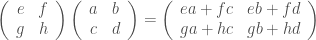
corresponds to the matrix $\left(\begin{array}{cc} a & b \\ c & d\end{array}\right)$ . In general, the number of columns of the corresponding matrix is the number of dangling wires on the left, and the number of rows is the number of dangling wires on the right. Moreover, the entry at row i and column j is the number of paths from the jth wire on the left to the ith wire on the right.

Finally, the composition

corresponds to the matrix obtained by performing the matrix multiplication ①.

And, as you’ve seen, it all follows from how adding and copying interact!

Continue reading with Episode 11 – From Diagrams to Matrices

9. Natural numbers, diagrammatically

We spent the last few episodes assembling our toolbox of equations. The game in graphical linear algebra is as follows: we consider two diagrams to be equal exactly when we can use the equations and graphical reasoning to prove it. If we cannot, we will consider them to be different. A mathematician would say that we are considering the free system on this set of equations.

If this idea is not clear, then imagine playing a board game: the things that you are allowed to do are only those that are specified in the rules. If something is not in the rules, then it is not allowed. Board game rulebooks typically do not include every possible way of how one could break the rules. People are way too creative at cheating; no wonder that law is such a complicated mess! In a similar way, we are usually not going to explicitly say when two diagrams are different: we consider them to be different if it is not possible to show, using the rules, that they are equal.

Anyway, here’s a convenient cheat sheet for the equations we have met so far, to save unnecessary clicking between episodes.

I hinted back in Episode 3 that graphical linear algebra has something to say about counting. That’s the plan for today. We will focus our attention on a very particular class of diagrams: those with exactly one dangling wire on the left and on the right. As it turns out, such diagrams are very closely related to natural numbers: that is, non-negative integers 0, 1, 2 and so on. For example it makes a lot of sense to associate the following diagrams with the corresponding numbers:

Remember the intuition about numbers travelling on wires? Well, associating numbers to diagrams is compatible with all that. For example, let’s consider sending a number x on the left dangling wire of the diagram that we are associating with the number 3.

The output is x + x + x = 3x. So, whatever the input, the diagram acts by multiplying it by 3. If you look at the diagrams for 0, 1 and 2, the idea is the same.

There is also a nice graphical intuition at play here: the number associated to a diagram is the number of paths from the dangling point on the left to the dangling point on the right. So, in the diagram to 0 there are no paths from left to right, in 2 there are two different paths, and so on. This graphical intuition is very important and we will come back to it again soon.

Although this is all quite cute, the correspondence between numbers and diagrams is not merely skin deep. As we will discover, the algebra of diagrams allows us to perform the basic operations of arithmetic: addition and multiplication. Thus, while our slogan so far is that linear algebra is all about what happens when adding and copying meet, we can actually be more extreme: even the basic idea of natural numbers is explained by adding and copying!

We start by defining a translation from numbers to diagrams, which will be useful for us as a syntactic sugar. The expression “syntactic sugar” is probably quite familiar to you if you are a programmer: it means a construction that is useful to have as part of your language, but that does not actually add anything new: the language does not become any more expressive. Syntactic sugar can always be translated away to phrases that we had before, but having it may be convenient for several reasons. This is exactly the case that we have before us.

Our syntactic sugar is a family of special diagram components, one for each natural number. We start with our good friend 0. We use the special := notation to indicate that we are actually defining the thing to the left in terms of things that we already know about.

The reason for the name (base) is that we will define the syntactic sugar recursively, and the definition above is the base case of the recursion. The recursive case is:

Maybe you have not seen the use of recursion before. It is something that many first year Computer Science undergraduates are very scared of; I know from personal experience! The reason is that, if you look at (rec), we are trying to define something (the left hand side), but we are using it again in the definition (the right hand side). This looks circular and weird — but don’t worry, it makes sense, and is not very difficult. The best way to get the hang of it is to experiment with some concrete examples.

So let’s understand the first few numbers, starting with 1.

We use (rec) to get the first equality, then (base), then (Unit), then (Counit). So the diagram that corresponds to 1 is simply the identity.

Let’s do 3 now.

We use (rec), then (rec) again, and then we use our knowledge of the diagram for 1, which as we have discovered above, is simply the identity.

It is important not to confuse the syntactic sugar for a natural number with a number travelling on the wire, as per our standard intuition. In fact, the sugar acts by multiplying its input by the number it represents, like so:

Let’s prove this!

But how does one prove something about all natural numbers? We could start showing that it holds for individual cases, say n = 13, but that would not be very satisfactory. Maybe we got lucky with that particular choice, maybe it’s not true for n = 12?

The trick is to use mathematical induction: if we show that the above is true for n = 0 (the base case) and whenever it is true for n = k then it is also true for n = k + 1 (the inductive step), then we can conclude that it holds for all natural numbers n. It’s kind of a bootstrapping process: how do I know that it’s true for n = 13492? Well, we know it’s true for n = 0. But because it’s true for n = 0, it must be true for n = 1, using the inductive step. But because it’s true for n = 1, it must be true for n = 2. And so on, until eventually we get to n = 13492.

We start with the base case, n = 0. Using (base) we need to check the behaviour of the following circuit.

And indeed, according to our established intuition about how the generators behave, a number x arrives on the left, is discarded, and a 0 is produced by the zero generator. But 0 = 0x, so the effect of the 0 sugar is to multiply its input by 0, as we are claiming.

Now let’s assume that this works as advertised for n = k and try to show that it holds for n = k + 1. The assumption is called the inductive hypothesis. For the k + 1 circuit, we use its defining equation (rec) and consider the behaviour of the following.

Again a number x arrives on the left, and is copied. The first copy is fed into the k sugar, which, by the inductive hypothesis, multiplies its input by k, resulting in the output kx. The second copy of x is untouched, and so kx and x are fed into addition, resulting in the output kx + x. But kx + x = (k + 1)x, which is what we want!

This concludes the induction and the proof. We will do many more induction proofs, so if all this is new to you then you will have plenty of examples to get comfortable!

We now move to the meat of this episode: showing how the algebra of diagrams can be used to express some familiar operations on numbers. Let’s start with adding: we willl prove that the following equality holds for all natural numbers m, n:

One way of understanding (sum) is that it show that ordinary, old-fashioned addition of natural numbers is already a part of our language: we can understand it with the basic operations of graphical linear algebra.

So let’s start by looking at what happens when n = 0, the base case of the induction.

We first use (base), then (Unit) and (Counit) together in a single step. Finally m = m + 0, as we all know. This shows that, no matter what m is, (sum) is true when n = 0.

Next, let’s look at the inductive step: remember, we can assume that what we want to prove, (sum), is true whenever n = k, and simply show that it is true for n = k + 1. Here we go:

First we use (rec), then (Assoc), then (CoAssoc). Next comes the use of our inductive hypothesis, and finally we use (rec) again. This completes the induction, and the proof of (sum).

We are going to prove a few more things in this episode. The first is the following useful equation, which holds for any number m.

Again the proof is by induction. For m = 0, it suffices to use (B4), the bone equation.

Next the inductive step.

First we use (rec), then (B2), then the inductive hypothesis, and finally (Counit). That’s (discarding) proved then.

The next property that we need is the following.

Let’s do the induction. For the base case, we have:

The proof of the inductive step is long, but not very complicated. We just need to apply (CoAssoc) a number of times and (CoComm) once to get the right alignment of the copies on the left. In the third step we use the inductive hypothesis. It is not super important to follow all the steps, so feel free to skip it.

If you did go through the proof carefully, maybe you spotted the one step where I cheated. It was the point at which I used (sliding) — remember that we are allowed to slide generators along wires. The reason why I was being slightly naughty is that the diagram for the number k is not, strictly speaking, a generator: it is syntactic sugar. However, because it is built from basic generators, one can show without too much difficulties that it can also be slid. In fact, it is not too difficult to show that any diagram whatsoever can be slid along wires.

Here’s a claim which I will not prove, because you have seen enough of examples of how to prove things by induction to be able to do it yourself. The claim is this:

For any natural number n, the bizarro version of the diagram for n is itself.

This is a useful fact to note, because we immediately get the following two things for free:

The reason why we know that (zero) and (adding) hold is because they are the bizarro versions of (discarding) and (copying). We can simply repeat each step in the proofs of (discarding) and (copying), but in the bizarro world.

We should spend a little bit of time discussing (adding), because it seems contrary to our expectation that the adding generator ought to be adding things. So why isn’t m + m = 2m? Well, let’s come back to our intuition of numbers on wires. Consider the left hand side of (adding), it has two dangling wires on the left on which we can send two numbers x and y. Next, remember from the introduction that the diagram for m acts by multiplying its input by m. Then the two outputs are fed into the adding operation, like so:

What about the right hand side? Performing the individual operations gives us the following behaviour:

But multiplication distributes over addition, so m(x + y) = mx + my; the behaviour of the two sides of (adding) is the same. We have, of course, already seen how to add natural numbers in graphical linear algebra, and it is handled by a combination of the adding and copying generators, as demonstrated in (sum).

There is just one more thing to prove in this episode, and it concerns another famous operation on natural numbers.

Just like (sum) can be understood as saying that ordinary addition of natural numbers can expressed using graphical linear algebra, (multiplication) is saying that ordinary multiplication of natural numbers is just composition.

To prove it—you guessed it!—we will use induction. The base case is the following, and we have the chance to use the (zero) property.

Next comes the inductive step, where we use both (adding) and (sum).

This completes the proof of (multiplication).

We have shown how natural numbers, addition and multiplication arise in graphical linear algebra. But there is one point about which you may be nervous: we have shown all kinds of useful properties, but what if actually 2 = 3 in graphical linear algebra? What if every number is equal to every other number? Maybe there is some crazy graphical proof that shows this? And how do we show that one cannot prove something, anyway? This is where the graphical intuition about counting paths comes in, and we will come back to this in the next episode.

Another question that you may have is the following. We have shown that all natural numbers can be understood as certain diagrams with one dangling wire on the left and one on the right. But are there some diagrams of this kind which are not equal to one that represents a natural number? In fact, this is not the case: this class of diagrams is in 1-1 correspondence with the natural numbers: every diagram with one dangling wire on the left and right is equal to one that comes from a number. There are several ways to show this, and we will explore some of these techniques in subsequent episodes.

Continue reading with Episode 10 – Paths and Matrices

Graphical Linear Algebra

Menu

Author Archives: pawel